Quadratic cones, point sources and vertex directions
Exposition and figure: GPT-6 Astra (OpenAI), October 2026. Original exposition: CC0. Supplied programme readings retain their stated credits and licences.
A quadratic cone is smooth away from its vertex. There, its singular directions come from a one-dimensional boundary value. At the vertex a point source can force every direction to be singular, whereas a homogeneous equation permits only characteristic directions. The signature determines which of these two mechanisms governs a normalized one-sided power. More general holomorphic boundary values also admit moving smooth arguments, with a precise distinction between regular and critical limiting maps.
The first classifications use ordinary smooth wavefront. Theorem 11 proves the same sets at analytic regularity and in every derivative-growth class defined below. Fourier transformation uses . Pairings are complex bilinear.
Scalar directions and the two boundary signs
Write
Here is the entire normalized family initially equal to . In particular and for . The boundary-power reading proves these identities as distributions.
Lemma 1 (scalar wavefronts). For every real ,
For every real ,
Proof. Corollary 3.2 of the boundary-power reading gives
The exponent at zero is greater than . For a compact smooth cutoff , the product-transform formula gives an absolutely convergent convolution with . If , its absolute value is at most
The last integral follows by ; it is finite for . Taking arbitrarily large excludes every negative direction. The distribution is smooth away from zero. It is not smooth at zero, since on it equals , which is unbounded as . The ordinary wavefront projection theorem therefore supplies a direction at zero; conicity leaves exactly the positive ray. Complex conjugation gives the negative ray for .
For the logarithm, choose near zero. Theorem 4.1 of that reading gives
The second term is smooth and compactly supported, since vanishes near zero. The first has rapid Fourier decrease on the negative ray by the preceding calculation. Fourier differentiation and division by there give the same decrease for . Its unbounded logarithm at zero supplies the positive ray. Conjugation again gives the lower sign.
Each is real, supported in , smooth away from zero and nonzero. At a negative integer it is a nonzero delta derivative. At every other real parameter it has the nonzero density on . If it were smooth at zero, its vanishing on the negative side would force every Taylor coefficient there to vanish. Taylor's estimate of order , compared with that density as , is impossible. A nonzero delta derivative is also not smooth: a continuous function supported at a point is zero. Thus zero is its singular base point. For a real cutoff and a real distribution, the Fourier values in opposite directions are complex conjugates. Regularity in one ray is consequently equivalent to regularity in the other. Projection and conicity give both rays. Reflection proves the assertion for .
Constructing the quadratic distributions through the vertex
Let , and let be a nonsingular real matrix. Define
Let be its positive and negative eigenvalue counts; thus . These counts include the definite cases. The differential is nonzero whenever .
For put . On punctured space the submersion pullbacks and are defined. Their degree is : the pullback composition law and give this scaling on tests. This degree is nonresonant and greater than . Let be their unique homogeneous extensions through zero. For define instead
These are locally integrable functions. Values on do not change them as distributions. The logarithm, rather than the constant power , is the two-dimensional point-source expression.
Lemma 2 (the actual boundary approach). For ,
For the corresponding logarithms converge to the in (Q5). All logarithms use argument in above the real axis and in below it.
Proof away from zero. Complete to smooth local coordinates . In them the upper argument is , with the positive smooth . We give a direct argument for every negative integer or half-integer .
If is not an integer, choose an integer with and set
Then , and extends continuously across the boundary, including zero, from the upper half-plane. If , take and
Differentiating first gives ; the next derivatives give . This is again continuous at zero.
On a fixed compact chart and for small , let
Repeated chain differentiation gives . Integration by parts therefore pairs the power against a test by pairing against of that test. The coordinate Jacobian is included in the test. The functions converge uniformly on its compact support, while these transposed tests converge in every smooth seminorm to . The limit is exactly applied in the coordinate: the same calculation with identifies its boundary trace. A finite partition covers every compact punctured support. Conjugation proves the lower case.
Proof at the vertex. For each fixed , the power in (Q6) has absolute value bounded by , so it is locally integrable and homogeneous of degree on the whole space. Its global value is thus the unique nonresonant extension of its punctured restriction. The weak continuity of that extension in the homogeneous-extension reading, Theorem 3.1, transports the proved punctured convergence to every test on . No point-supported term is discarded.
For the logarithm write and . The upper logarithm is
At a zero of its tangential derivative on the sphere is , since ; it is nonzero. Coordinate completion on the sphere therefore makes each such zero a regular surface. In those charts is integrable, by ; a finite cover handles the compact sphere. Where , it is bounded locally. For ,
off the measure-zero set : its argument is bounded by , its positive real part is bounded on the compact sphere, and its negative real part is at most . The radial bound now proves local integrability and dominated convergence to (Q5), using the full polar Jacobian. The definite case has no angular zeros and the same argument is simpler. Conjugation gives the lower limit.
The exact source and its signature
Let be the sphere area, and put
Theorem 3 (quadratic boundary sources). On the whole space,
In particular the coefficient is nonzero for every signature.
Proof of the complex identity. For a complex symmetric with , let be the determinant branch proved in the point-source reading, and let use as in (Q4). We first establish
For real positive , diagonalization supplies and . The test-level linear chain rule gives , while . The point-source reading proves and . These prove (Q8) for all real positive .
Both sides paired with any compact test are holomorphic in the independent complex entries of . Here is the integrability justification. On a compact subset of the positive-real-part domain, . Every parameter derivative of the power is bounded by a constant times , since each differentiating quadratic numerator cancels the degree of its additional denominator. This is locally integrable. For the logarithm the undifferentiated bound is ; every positive parameter derivative is bounded. The adjugate formula gives holomorphic, locally bounded derivatives of . Dominated difference quotients give coordinate holomorphy and joint continuity of the pairings; the polydisk proof in the complex-quadratic reading gives joint holomorphy.
In a small polydisk about , the paired difference in (Q8) vanishes when all entries are real and close to those of . Apply the one-variable identity principle successively to each independent entry, keeping the others real until their turn. The difference vanishes on that polydisk. The domain is convex. For any target , restriction to the complex parameter line , on a connected neighborhood of the real segment , propagates this zero to . This proves (Q8) throughout the domain.
Proof of the boundary constant. Set . The determinant-branch lemma gives
For , with , the branch relation is
Multiply (Q8) by , and use Lemma 2 and coefficient convergence. The limit on the left is . Dividing by , the phase on the right is
Convergence with the varying differential operator is legitimate: each fixed derivative of the convergent distributions converges, and each matrix coefficient converges.
For , the logarithm relation has the additive constant . Its derivatives vanish, so the same limit of the second line of (Q8) gives the phase
.
The real coefficients of and complex conjugation give the lower sign in every dimension.
Theorem 4 (one-sided source coefficients). With the defined above, for every ,
Thus the first coefficient is nonzero exactly when is odd, and the second exactly when is odd.
Proof for . At the scalar identities are
We verify all parameters needed here without assuming a reflection formula. At , the ordinary integrable boundary values on the two half-lines and give
and
.
At , the proved jump gives both identities. Differentiation gives
Together with and
, these prove (Q11) by induction down each of the two parameter sequences. Those sequences contain every , .
Pull back (Q11) on punctured space and extend homogeneously. Linearity and uniqueness of the degree- extension give the same identities with . Apply Theorem 3. For the positive side the difference of phases gives
Gamma recurrence and the sphere constant give
;
the sine is . The second line of (Q11) gives
.
These are exactly (Q10).
Proof for . Formula (Q5) gives
Theorem 3 consequently gives coefficients
and its negative. Since ,
, proving (Q10).
Every wavefront covector, including the vertex
Use the following subsets of :
Theorem 5 (the full quadratic wavefronts). For every nonsingular real symmetric and every ,
The first line uses the logarithmic when . Empty quadratic cones and empty null fibers are allowed.
Proof away from the vertex. Since there, the exact submersion wavefront equality (WF15) and Lemma 1 give precisely for and for . These distributions are smooth where . Thus no nonvertex covector has been omitted or added.
Proof at a nonzero point source. A finite constant-coefficient differential operator cannot enlarge ordinary wavefront. To recall the local argument, choose cutoffs inside a neighborhood on which a compact representative of has rapid decay in a cone. Smooth localization gives that same decay, on a smaller cone, for every smooth compact multiplier there. The identity
then proves the derivative inclusion: its first term acquires only a Fourier polynomial, and the second is another localized multiplier. Iterate and take finite sums. Also every cutoff equal to one near zero leaves . Hence
Theorem 3 applies this to each . The nonzero cases of Theorem 4 give the odd-signature cases for .
Proof when the source vanishes. In an even-signature case, Theorem 4 gives everywhere. The analytic differential regularity theorem applies to this constant-coefficient operator, whose symbol in the convention is . It gives
This proves the required upper bound at zero, including when is definite.
For the lower bound retain any with , and let
Each , so the already proved full nonvertex conormal formula contains , with multiplier . Ordinary wavefront is closed in the punctured cotangent bundle; its complement is open directly from the cutoff-and-cone definition. Letting , while retaining the same nonzero , gives . This proves every point of . Together with (Q15) it proves equality and completes all cases.
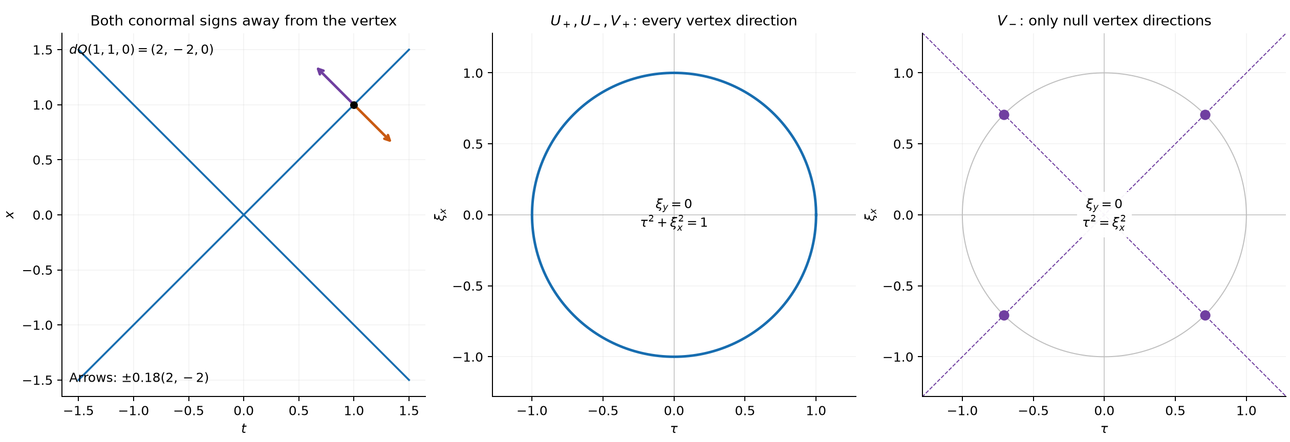
For , the left panel shows the base section and the two normal signs at ; the displayed normal arrows are scaled copies of . The other panels show unit covectors in the section , not the whole three-dimensional fiber. The boundary values and the positive-side have every vertex direction. The negative-side has exactly the null ones; in this section they are the four points . Theorem 5 proves the complete sets. Reproducible figure source.
Corollary 6 (all forward wave powers and speeds). Put
Then , and
The backward kernel obtained by has the same full vertex fiber and the corresponding cone.
Proof. For , the exact linear chain rule gives
, and .
Iteration proves the displayed source identity, with the factor retained for every . At each nonzero forward cone point, the local formula has a nonzero constant and the scalar family of Lemma 1. Its exact submersion pullback therefore has both conormal signs. Away from that cone and the vertex the kernel is smooth: its interior formula is a smooth power, or zero at a delta-derivative parameter, and it vanishes outside its supporting cone. Finally (Q14), applied to , gives every nonzero vertex covector. Coordinate covariance transports the cone differential to . Time reflection has absolute determinant one, preserves the source and gives the backward statement.
Boundary values along arbitrary smooth approaches
The boundary limit also survives a moving complex argument. The hypotheses concern its real limiting map and its convergence in the smooth topology; the height need not be proportional to the parameter, and the real part may move.
We use Cauchy kernels and distributional boundary limits, Theorem 3.1 and Corollary 3.2, for the horizontal boundary distribution on finite-regularity tests. Gluing holomorphic sides, Lemma 1.1, constructs an -fold primitive with logarithmic growth. The exact submersion construction is the supplied smooth pullback reading, Section 18.5; its completed coordinates and Jacobian are supplied by the coordinate-completion lemma cited at the start of this lesson.
Let be an open interval, let , and set
Let be holomorphic on . On each compact interval , assume a bound
where is a nonnegative integer and . Larger compact intervals may require larger integers. These local bounds give the boundary distribution .
Lemma 7 (a continuous primitive at the boundary). Locally near any compact subinterval, choose a slightly larger interval on which (A2) holds with exponent , and put . There is a holomorphic , continuous up to that real interval, such that
In particular, this representation acts continuously on compact tests.
Proof. The gluing lesson's Lemma 1.1 constructs a holomorphic with and
uniformly on each retained compact horizontal interval. For , take ; its boundedness implies the displayed, weaker bound. Choose a reference point and height inside a slightly larger rectangle, and define
The fundamental theorem and give and , exactly as in that primitive construction. Thus is holomorphic and .
The second integral in (A5) converges at , uniformly in the retained horizontal interval. Indeed,
The equality follows by integration of ; the limit follows, for example, by writing and comparing with the exponential series. Hence converges uniformly to a continuous function . Continuity of that limit and the same uniform estimate prove joint continuity at the real boundary.
For a compact test , horizontal integration by parts gives
There are no end terms. The horizontal boundary theorem identifies the left limit with . The right side is bounded by a compact-interval constant times . This proves (A3) and its stated test continuity.
Theorem 8 (moving-map boundary limit). Let be open, , and let be smooth with everywhere. For each , let be smooth and complex valued, with
Then
More precisely, on every fixed compact test support , there are an integer , a constant , and numbers such that
for all sufficiently small and all smooth tests supported in . These pairings extend to compact tests. Consequently the convergence is uniform on bounded sets of smooth tests, and permits moving tests converging in that fixed norm. The corresponding statement holds for approaches from the lower half-plane and .
Proof in completed coordinates. Since , complete to coordinates in a neighborhood of any point. Use a compactly supported local test and a slightly larger such chart. Replace by its expression in these coordinates; it converges to in every smooth seminorm. The test becomes
The absolute Jacobian is essential. It is smooth and positive on this chart. Every test derivative through any fixed order is bounded by a constant times the corresponding finite norm of , by the product and chain rules. Its support lies in one fixed compact set.
The real projections of of that compact set lie in one retained interval for small , and their imaginary parts tend uniformly to zero from above. Choose the continuous primitive of Lemma 7 on a larger rectangle, and write . On a neighborhood of the test support put
The denominator tends to with every derivative, so it is nonzero there for small , and in every smooth seminorm. The transpose is bilinear: there is no complex conjugation of .
The complex chain rule gives
.
After integrations by parts,
Only is integrated by parts, and compact support removes each end term.
Here are estimates uniform in the test. Expanding the finite product of first-order operators gives
To justify these expansions, start from
.
An induction writes its -th power as a sum of derivatives , , with coefficients that are finite sums of products of derivatives of through order . Differentiating once and using the product rule proves the next step. All coefficients are uniformly bounded on the fixed support, and converge to those of , because in . Multiplying their supremum bounds by the finite support volume proves (A14).
Uniform continuity of on the relevant closed rectangle gives
Subtract from (A13). Equations (A14) bound the difference by
The limit integral, by (A7) and integration in , is
This is precisely the previously constructed submersion pullback in completed coordinates, including its absolute density factor. No value of on the real axis has been substituted into a singular expression.
Localization and the test topology. Cover by finitely many such charts and use a fixed smooth partition. If their growth exponents differ, take the largest of their finite test orders. Each partition multiplier and coordinate change is continuous in that finite norm. Summing (A15) gives the first estimate in (A10); boundedness of , (A14), and the corresponding limit integral give the second. The submersion pullbacks agree on overlaps by their proved coordinate construction, so the limit is on all of .
The same formulas extend continuously to tests with fixed support, by the supplied finite-norm smoothing approximation; equivalently one may integrate by parts directly for those tests. If in with common support, the common bound controls the pairing with , and the fixed-test difference tends to zero by (A10). A bounded smooth test set has a common compact support and bounded norm, so (A10) proves strong distributional convergence. For the lower side apply the upper theorem to , the maps , and the submersion . Reflection and the already proved pullback composition law identify the limit with .
No estimate of the form occurs in this proof. In particular, a jointly smooth map with , nonzero , and positive-height values satisfies (A8) on each compact set and therefore (A9). This includes arbitrary smooth real drift and heights flat at .
Corollary 9 (critical points over regular boundary values). Retain the hypotheses on and , but allow at some points. Suppose that at every such point , extends holomorphically to a complex neighborhood of , agreeing with its original values above the interval. Then still has a distributional limit. Near regular points it is the submersion pullback of Theorem 8; near each critical point it is the smooth function given by the holomorphic extension composed with .
Proof. Around a critical point, shrink the source neighborhood so that the image of its closure under lies in a compact subset of the extension domain. For small , its image under remains in that domain. Uniform continuity of each derivative of the extension on a slightly larger compact set, together with the finite chain rule and (A8), gives convergence in every smooth seminorm to the extension composed with . Around regular points Theorem 8 applies. On an overlap the local distributional limits coincide, since they are limits of the same functions against every test there. A finite partition on each compact support therefore defines the global limit, with the local finite-test estimates already proved. This argument asserts no pullback at a critical point lying over a singular boundary value.
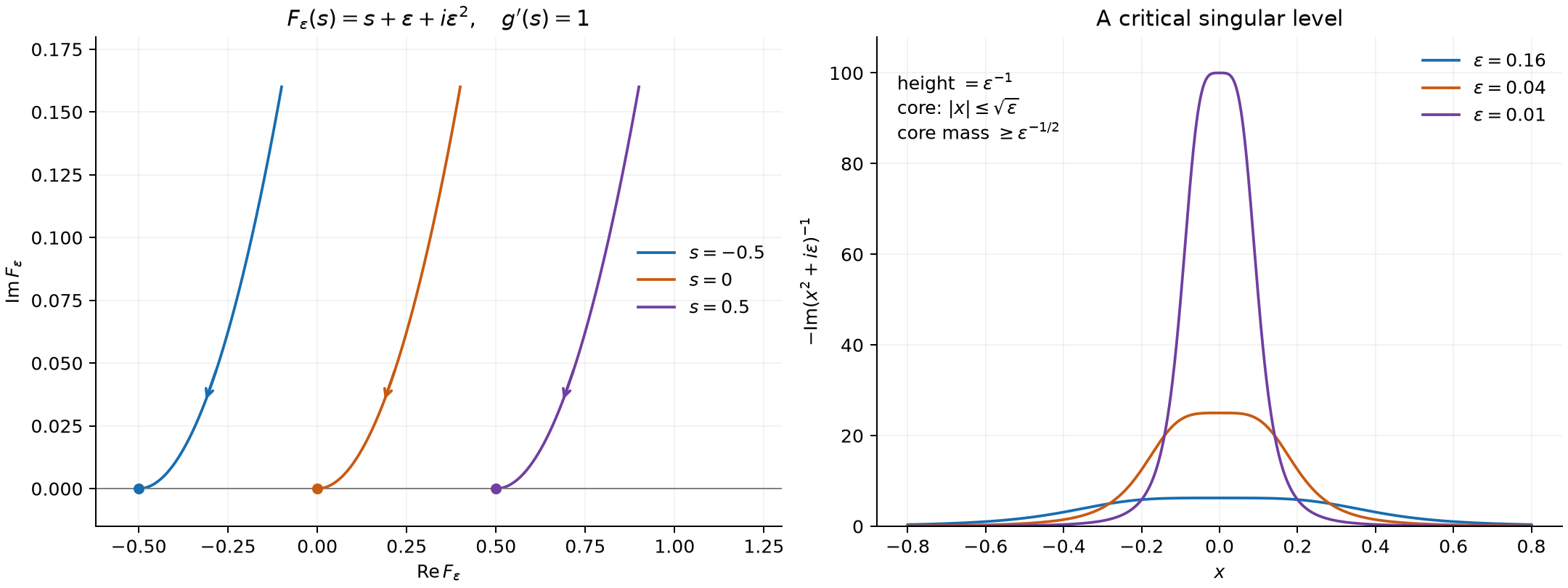
Left: the paths , for and , end at a real map with derivative one. Theorem 8 preserves the boundary distribution despite the real drift and changing height. Right: the exact profiles , at , have height and a core width proportional to . Exercise 8 proves divergent mass near the critical point; the plotted samples are illustrations of that proof. Reproducible figure source.
Analytic directions and every derivative-growth class
Fix any nondecreasing sequence , , . These hypotheses are the derivative-growth convention of that reading. In particular they include , . Its comparison theorem gives
For the second inclusion, the analytic sequence is at most for ; the harmless constant is absorbed into the witness estimate.
Lemma 10 (analytic scalar boundary signs). Every equality in (Q2)–(Q3) holds with replaced by , and also by .
Proof. For real , choose the holomorphic branch in the upper half-plane, with argument between zero and . At , ,
On , this is bounded by for any integer . The boundary-power construction identifies its boundary as . The dual of the positive imaginary ray is the nonnegative frequency ray in our Fourier convention. The cited boundary theorem therefore excludes all negative analytic directions.
The same theorem applies to the upper logarithm. On a bounded real interval and , its argument is bounded by , its positive logarithmic part is bounded, and its negative logarithmic part is at most . Consequently
The last inequality follows, for example, from
.
The boundary is , by the earlier logarithmic limit. Thus it too has no negative analytic direction.
Both boundary functions are real analytic away from zero, including on the negative real half-line: near each nonzero real point their chosen branch has a holomorphic extension to a small disk avoiding zero. One can construct that local branch by the convergent logarithm series about the point, choosing its constant to match the upper value. The local analytic-function criterion therefore excludes every covector away from zero. Lemma 1 and (B1) force the positive ray at zero. This proves the upper-sign equalities. The lower branches satisfy the same polynomial bounds on the lower half-plane, whose imaginary cone has nonpositive dual; the same argument, with Lemma 1's lower ray, proves their equalities.
For every real , is analytic on each open half-line. At a negative integer it is supported at zero; otherwise its nonzero half-line density is a constant multiple of , an analytic function there. Hence its analytic wavefront is contained in the full punctured fiber at zero. Lemma 1 and (B1) already include that whole fiber. Finally (B1) places every intermediate between two equal sets in all these cases.
Theorem 11 (the quadratic and causal classifications in every class). For the distributions of (Q4)–(Q5), all three sets
, and
are equal, with the exact values in (Q13). The same assertion holds for every forward or backward in Corollary 6, with its exact set (Q17).
Proof for quadratic distributions. On punctured space is an analytic submersion. Lemma 10 and exact analytic submersion covariance give precisely for , and for . Where the local formulas are analytic, so these exhaust the nonvertex analytic directions.
At the vertex, each , and each odd-signature specified in (Q13), already has the entire punctured smooth-wavefront fiber by the nonzero source identity. Inclusion (B1) gives the entire analytic fiber as well. A fiber has no additional nonzero covectors to include.
In the remaining signature cases on the whole space. The analytic differential regularity theorem used in (Q15) gives the analytic upper bound . The exact path (Q16) and closedness already give every one of these covectors in smooth wavefront. Thus the analytic and smooth fibers agree here too. This argument includes definite forms, for which the nonzero null fiber is empty, and the logarithmic two-dimensional cases. It uses the whole-space source identity at zero, not a nonexistent submersion at that point.
Proof for causal powers. At a nonvertex forward cone point, and . The local formula in Corollary 6 is a nonzero scalar multiple of an analytic submersion pullback of , with . Lemma 10 gives both conormal signs exactly. In the cone interior the ordinary power is analytic; at negative integral parameters the scalar distribution vanishes there instead. Outside the cone the kernel is locally zero. Points with other than the vertex also have a neighborhood disjoint from the supporting cone. Thus there are no other nonvertex analytic directions. At the vertex the equation supplies the full smooth fiber by (Q14), hence the full analytic fiber. Time reflection is an analytic diffeomorphism, so it proves the backward assertion. Finally (B1) gives every stated intermediate class.
The distinction between a homogeneous equation and a point-source equation remains essential at analytic regularity. Characteristic directions bound the former. The latter can have a full vertex fiber even when nonvertex conormals have only characteristic limits.
Proposition 12 (analytic coordinates and nonvanishing weights). Let be an analytic diffeomorphism, let be a nowhere-zero complex-valued real analytic function on , and let be any distribution in Theorem 11, restricted to . Put . Then
Proof. Analytic diffeomorphism covariance gives equality for and ; the supplied smooth covariance gives it for . Multiplication by gives inclusion for each class. Its reciprocal is real analytic locally: extend its power series holomorphically, shrink until it stays nonzero, and expand by the geometric series about its value at the center. Multiplication by that reciprocal gives the reverse inclusion. For smooth wavefront the same reciprocal is smooth. Theorem 11 therefore gives (B4). No assertion about a weight at one of its zeros follows from this argument.
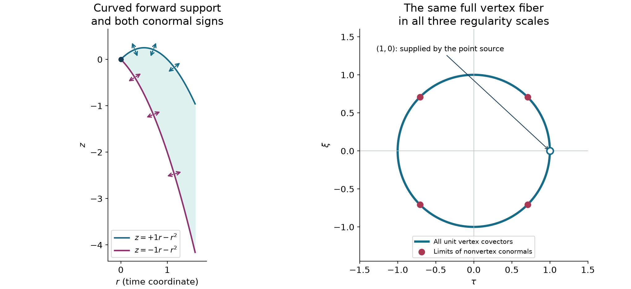
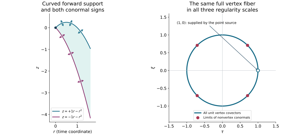
The left panel uses the analytic map . Its forward cone boundaries are , . The displayed arrows are normalized samples of both signs of the exact covectors ; they represent covectors in these fixed Euclidean coordinates, not propagation velocities. At the origin, the right panel shows every unit covector. The four marked null directions are only the limits of nonvertex conormals. Exercises 10–11 prove the formulas and the strict distinction. Vector figure · Reproducible figure source.
Exercises with complete solutions
Exercise 1 (foundation: the three-dimensional saddle). Take . Compute all four point-source coefficients and compare the vertex wavefronts of and .
Solution. Here , , , and . Since and ,
The normalized powers are the locally integrable functions
.
Both have every nonzero conormal over each nonvertex cone point. At the vertex has every nonzero covector, whereas has exactly
, with the joint zero removed. Its nonzero interior values on do not introduce any wavefront there, since they are smooth. These are the sets displayed in the figure's sections.
Exercise 2 (intermediate: a cone delta with no point source). Let . Identify and , compute their source, and give their vertex wavefront.
Solution. Now , and both scalar families equal . Thus is the unique degree- extension of the punctured pullback . The notation specifies that extension; it is not an unsupported pullback at the critical point. The signature is , so both sines in (Q10) vanish. Consequently , with . The vertex fiber is precisely the nonzero set
.
The full wavefront also includes every nonzero multiple of over every nonvertex cone point. In contrast, each has source and a full vertex fiber: , and its determinant phase is again . Subtracting the two boundary-source equations agrees with the zero source of the delta term in their boundary jump.
Exercise 3 (intermediate: verify the logarithmic source directly). In two dimensions take . Check the constants in Theorems 3–4 using characteristic coordinates.
Solution. Set , . Then , , and the coordinate determinant has absolute value two. Almost everywhere,
Each mixed derivative on the right is . Returning to gives
.
Therefore , and . Also
as locally integrable functions. Its mixed derivative is zero, since each summand is independent of one variable. Formula (Q5) hence gives
These agree with in (Q7). All four distributions have a full vertex wavefront. Away from the vertex, the logarithms have their respective single normal signs, while the Heaviside distributions have both signs.
Exercise 4 (advanced: the definite cases are part of the theorem). For , determine and their wavefronts in every .
Solution. The negative-side pullback is zero off the origin. Its unique homogeneous extension is zero for ; for , almost everywhere. Thus in every case. For odd , the positive-side value is
Its denominator is finite and nonzero, as follows from the half-integer Gamma recurrence. The coefficient in (Q10) is nonzero, and its wavefront is the full vertex fiber. For even , is a negative integer, so the scalar is supported at zero. Its pullback on punctured space is zero because there; uniqueness again gives . Finally gives . All even-dimensional cases therefore have empty wavefront. This is exactly (Q13): the nonvertex cone and the nonzero null fiber are empty for a definite form. The logarithmic in dimension two still have a point source and a full vertex fiber.
Exercise 5 (advanced: retain an anisotropic determinant). Let . Compute the source coefficients, the dual null cone and the nonvertex normals.
Solution. The coordinate map has absolute determinant six. Thus , , and
Theorems 3–4 give
These are also the constants of Exercise 1 multiplied by , the pullback factor of a point mass. Nonvertex normals are multiples of
at . The retain respectively positive and negative multiples there and all vertex directions. The retain both signs there; at zero has every direction and has precisely , with zero excluded. For every such nonzero covector, the exact path from (Q16) verifies the limiting lower inclusion without replacing by an unrecorded normalized form.
Exercise 6 (foundation: a height flatter than every power). For , set
Determine the distributional limit of . Determine also the limit when the sign of the imaginary part is reversed, and for the upper approach with limiting real map .
Solution. The imaginary part in (A17) is positive. On each compact set every -derivative of tends to zero; thus (A8) holds with . Theorem 8 and the previously proved pole limits give
For a fixed strip height , the maps lie in that strip when . Reversing the imaginary sign gives
.
The height has no positive lower bound by , for any fixed and . Indeed, with , the quantity tends to zero: choose an integer in . Defining the exponential factor to be zero at gives a smooth function there. Repeated differentiation for has the form a polynomial in times ; the same bound makes each derivative tend to zero, and the fundamental theorem successively identifies the extensions as derivatives at zero. Hence this is also a jointly smooth approach, with all height derivatives zero at the boundary.
For the upper approach
,
the limiting map is reflection. The scalar identity
, , gives
The delta coefficient retains its sign because scalar distributional pullback uses the absolute Jacobian. The same result follows by reflection in Theorem 8.
Exercise 7 (intermediate: two simple level zeros and one harmless critical point). Let
Find the distributional limit of on the whole real line, including and the two roots of the limiting real map.
Solution. The maps approach in the smooth topology. Their positive heights are at most . The sole critical point of is zero, whose image is ; the function is holomorphic near that image. Corollary 9 therefore applies at zero, giving the ordinary smooth limit there. At each of the roots , , so Theorem 8 and the pole formula apply. They give
Here are the real principal-value and density factors explicitly. The pulled-back delta has coefficient at each root, by the one-dimensional change-of-variables test formula. The pulled-back principal value is the limit of
.
To identify it, use
Near , write , so . The endpoints removed by satisfy
.
This follows directly by solving the two quadratic equations, or by Taylor's formula for their local inverse, whose derivative has magnitude . Replacing these endpoints by the symmetric endpoints changes the singular integral by : the endpoint differences have length , and the integrand has size on those small intervals. The remaining local term is bounded. Thus the level-deletion limit is exactly the displayed combination of ordinary principal values. Away from the two roots it is the ordinary function. These local descriptions agree on overlaps and establish (A21) globally, without treating the critical point over as a singular level.
Exercise 8 (advanced: concentration at a critical singular level). Show that the smooth upper approach does not give a distributional limit for . Explain why this does not assert failure for every holomorphic at every critical map.
Solution. Choose a nonnegative compact smooth test , equal to one on , . Direct algebra gives
For and , the denominator is at most . Hence
A distributional limit would have a finite limit on this one fixed test, so it cannot exist. Both the nonzero-derivative hypothesis of Theorem 8 and the holomorphic-extension condition at the critical image in Corollary 9 fail at zero. The figure shows the exact concentration profiles in (A22); the inequality above proves the divergence for every sufficiently small parameter, independently of those samples.
For contrast within this same calculation, has no singular boundary value: smoothly, although the limiting map remains critical at zero. Thus the submersion condition is sufficient for all the admitted boundary functions, and cannot simply be dropped for that entire class; it is not necessary for each individual regular function.
Exercise 9 (foundation: a zero of an analytic weight). For an integer , determine the smooth, analytic and derivative-growth wavefronts of . Explain the role of the nonvanishing assumption in Proposition 12.
Solution. The boundary-power construction gives in distributions. On each compact test support these distributions have a common finite-order bound, by the boundary estimate. The multipliers tend to with all derivatives there. Pairing the difference against a fixed test thus tends to zero by that common bound. Since the product before taking the limit is identically one,
This function is analytic and every one of its wavefronts is empty. In contrast, Lemma 10 gives the positive ray at zero for in all three classes. The analytic weight has a zero at exactly that base point; its reciprocal is unavailable there. Thus analytic multiplication always gives the inclusion, but need not give equality at a zero.
Exercise 10 (intermediate: an analytic bending of a causal cone). In one space dimension with speed one, let be the forward wave kernel of Corollary 6. For , compute all three wavefronts of
Give its locally integrable density and the exact covectors on its two curved boundary branches.
Solution. The inverse is ; both maps are polynomial and their Jacobian determinant is one. The causal formula for is
almost everywhere. Consequently
The zero-measure boundary does not affect this locally integrable density. The weight is nowhere zero and analytic. Since
Proposition 12 gives the nonvertex pairs with , , , together with the entire punctured fiber at . There are no other pairs. On the branch , , the covector is
Its pairing with the tangent is zero. Both signs of every nonzero multiple occur. This proves the formulas displayed in the figure for smooth, analytic and every admitted derivative-growth wavefront.
Exercise 11 (advanced: what closure of the punctured cone misses). For the distribution in Exercise 10, determine the fiber at zero of the closure, in the punctured cotangent space, of its nonvertex conormal set. Compare it with the actual wavefront fiber.
Solution. Write the nonvertex covector on branch as
If these covectors tend to a finite nonzero as the base tends to zero, pass to one branch along a subsequence. The second component shows that has a finite limit ; the first then has limit . The limit is nonzero only if . Conversely, take for any and let . The resulting fiber is exactly
It has four directions on the unit circle. The actual wavefront at zero, by Theorem 11 and (B4), is the whole punctured plane: the point source supplies the other directions. For example is in all three wavefronts and is absent from this conormal closure. Taking the closure is necessary to retain the limiting null covectors, but cannot replace the separate vertex argument.
Fourier transforms on the dual quadratic cone
Throughout this section , , and have the meanings in (Q4). Write , , so that . We use the positive constant
where is the point-source constant in Theorem 3. The sphere and Gamma foundations prove the equality. The Fourier transform remains , with bilinear distributional transpose.
The passage to the boundary must control Schwartz tests at both zero and infinity. Order, positivity and distributional limits, Theorem 5.1, supplies a common finite order for a convergent sequence on a fixed compact test support. Compact factors and homogeneous equations, Proposition 3.1 and Theorem 3.2, supplies Fourier dilation and the annular construction of tempered extensions. The following estimate gives the particular continuity needed here.
Lemma 13 (homogeneous limits on Schwartz tests). Fix a real . Suppose that are globally homogeneous distributions of degree , and their restrictions to converge in to . Then has a unique globally homogeneous extension of that degree. Every and is tempered, and
One finite Schwartz seminorm bounds all these distributions.
Proof. Passing the dilation identity to the limit on each compact test proves homogeneity of . Theorem 3.1 of the homogeneous-extension lesson gives its unique extension, since is nonresonant. Choose a smooth cutoff , equal to one on the unit ball and zero outside the ball of radius two, and put . Its support lies in . Telescoping gives for . Homogeneity gives the annular identity
for any one of , initially on compact tests. These annular terms sum to . Indeed the unsummed small ball has the form , which equals
.
The finite-order bound for this fixed on the ball of radius two makes the latter tend to zero. For a compact test the large-ball cutoff is eventually identically one on its support.
Apply Theorem 5.1 of the distributional-limits lesson on to the convergent restrictions, including the limit. There are one order and one constant such that their absolute pairings with any test supported in are at most . Define
Product differentiation in (F3) then gives
For the second inequality on ; each derivative on the rescaled test contributes at most . For the first all such factors are at most one. Choose an integer . Both geometric tails are summable, uniformly in . Thus the annular series defines a continuous functional on , agreeing with on compact tests and bounded by . Compact-test density in , proved in the Fourier foundations, gives uniqueness. For each fixed the compact annular pairing converges. First make both uniform tails small and then pass to the limit in the finite middle sum. This proves (F2).
Let and denote the quadratic distributions already constructed, respectively from and . On the punctured frequency space . Define
These extensions are unique because . Their restrictions are homogeneous of degree by the scalar boundary law and the quadratic dilation. Lemma 13, or the annular tempered-extension theorem, makes them tempered on the whole frequency space.
Theorem 14 (both quadratic boundary transforms). For every real nonsingular symmetric in dimension ,
The identity holds on all Schwartz tests, including tests meeting the vertex of the dual cone.
Proof. Set , . Its real part is positive definite. Theorem 1.2 of Complex quadratic powers and the Cauchy kernel, with its exponent , gives the whole-space identity
Here is the canonical square root of the determinant, positive on positive definite real matrices. The cited theorem proves the two absolute integration interchanges on Schwartz tests, so (F7) includes frequency zero.
Put . Since , its inverse quadratic is . In a real orthogonal eigenbasis of , with nonzero eigenvalues ,
Also in every smooth seminorm on compact sets. The lower-half-plane version of Theorem 8, applied to and the submersion , proves
on the punctured space. Each reciprocal is a locally integrable global homogeneous function of degree : for fixed , (F8) bounds its absolute value by . Lemma 13 upgrades this to convergence to on Schwartz tests. Formally, apply that lemma along every sequence ; failure of any scalar test limit would supply a sequence contradicting the lemma.
On the physical side, the principal argument of lies in when . Multiplication by subtracts without crossing the branch cut, so
For fixed these functions are locally integrable, homogeneous of degree . Lemma 2 and Lemma 13 give the Schwartz-test limit . The determinant branch proved in Lemma 2.1 of the Gaussian lesson gives
Taking (F7) to the limit is legitimate because the Fourier transform maps each Schwartz test to a Schwartz test. Since , the total phase after solving for is
using . This proves the upper sign. Complex conjugation satisfies
, by the test-transform definition. Each quadratic distribution is even: reflection preserves its punctured definition and homogeneity, hence preserves the unique extension. Moreover and , first off the vertex and then by uniqueness. Conjugating the upper identity with the required reflection proves the lower one.
Principal values and the measure on the dual cone
Theorem 15 (one-sided powers and cone mass). Define the canonical homogeneous distributions
On the punctured space these are respectively the submersion pullbacks of and . On the whole space,
and the normalized one-sided powers have transforms
The distribution is a positive locally finite tempered measure. Writing on the unit sphere and , it is given by
If is definite, this measure is zero. If is indefinite, its support is the entire dual null cone , including its vertex.
Proof of the transform identities. The scalar boundary formula
, proved in the boundary-power lesson, proves (F12) off zero. There it also gives (F13), since and . The two sides of each identity are homogeneous of degree zero. The uniqueness of nonresonant extension from the punctured space proves their equality globally; it excludes an additional point-supported term.
Equation (Q11), whose scalar identities are proved in Theorem 4, gives
Use (F6), , and . In the first identity the coefficient of is
;
the coefficient of is
.
The second identity gives the corresponding phases with directly. Finally substitute and ; and give the real forms in (F14).
Proof of the measure formula. On the spherical gradient is , because its radial component is . It never vanishes. Theorem 1.1 of Regular level sets and transverse convolution gives the density on the punctured cone. To express that density radially, take a local parametrization of . The cone chart is . Since , differentiating this identity gives . Its Gram matrix is therefore block diagonal, with radial entry and angular block . The surface density is , while . Division gives (F15), by the exact surface-coordinate change formula of that theorem and a finite chart partition. This computation is in regular coordinates away from zero; it does not assert a submersion pullback at the vertex.
The compact regular hypersurface has finite induced measure, by a finite smooth graph cover and the surface integration formula. Its gradient norm has a positive minimum. Consequently (F15) is bounded near zero by . At infinity a Schwartz seminorm with exponent bounds the integral by . Thus it defines a positive tempered measure on the whole space. A radial substitution proves degree , and uniqueness identifies it with . If is definite then is empty. Otherwise eigenvectors of both signs give a nonzero null vector by balancing their squared coefficients, so . The positive smooth density has support all of , and radial integration gives every nonzero point of the null cone. Every neighborhood of the vertex contains such points with positive measure. This proves the support assertion.
For an indefinite form, (F14) has a useful parity interpretation. If is odd, is a nonzero multiple of , of support all of . If is even, it is a nonzero multiple of , of support exactly the dual cone. The same assertion holds for with . To check the full support of , every nonempty open set meets : a nonzero polynomial cannot vanish on an open ball, by its finite Taylor expansion. On that set , which a sufficiently small test of constant sign detects. Both spectral alternatives therefore have exactly the stated supports.
Corollary 16 (normalized fundamental solutions). Put
Then , and
The difference is a solution of . It vanishes precisely when is definite.
Proof. Theorem 3 and (F17) give the point source. Equation (F6) and give the first transform in (F18), and (F12) gives the other two. Fourier differentiation gives the multiplier for ; (F13) also verifies both the source and the homogeneous equation in frequency space. Fourier injectivity from the supplied inversion theorem, together with the zero and nonzero alternatives for , proves the last assertion.
These boundary choices do not select a direction of physical time. Both are even under simultaneous reflection of all physical coordinates. A causal fundamental solution requires its separate support condition, as in the earlier causal constructions.
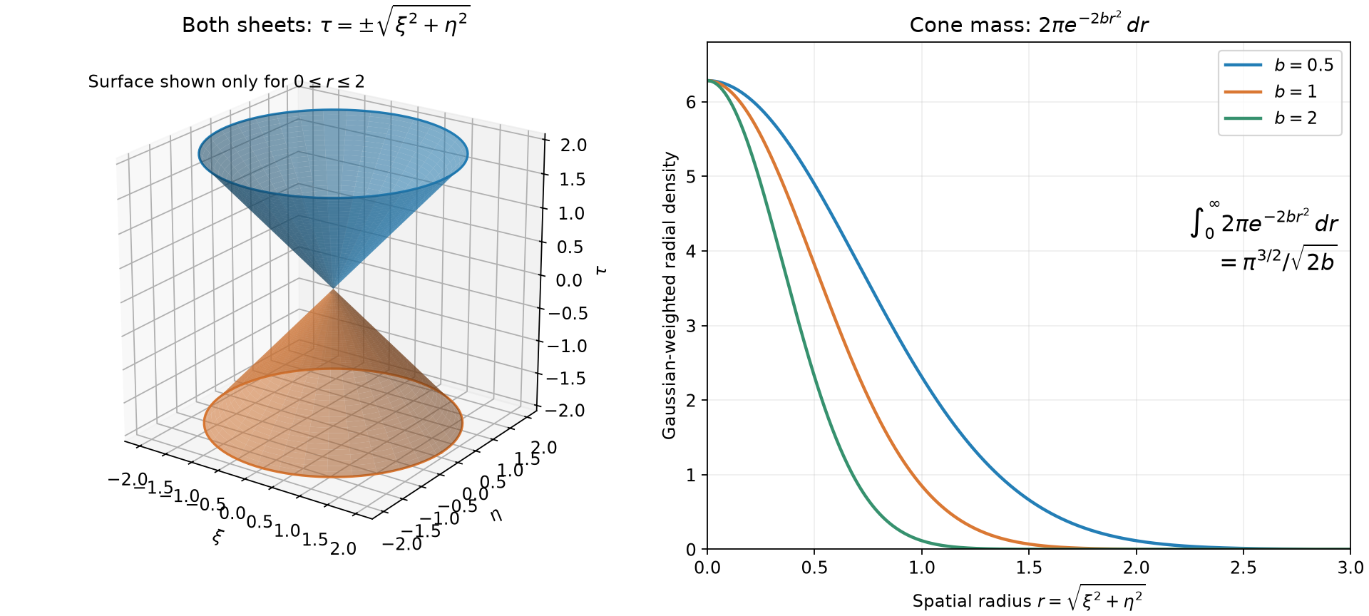
Figure. For , the left panel displays both sheets , , truncated at . The right panel shows the exact radial densities of the Gaussian-weighted cone measure for three positive . Here is the spatial radius and the Euclidean radius on the cone is . The support is proved in Theorem 15; the density and its integral are proved in Exercise 17. Reproducible figure source.
Exercises on quadratic Fourier transforms
Exercise 12 (basic: a three-dimensional saddle). Let . Compute the transforms of and recover the two point-source equations for by Fourier differentiation.
Solution. Here , , and . Equations (F6) and (F14) give
The Fourier multiplier of is . By (F13), multiplication of the last two expressions by gives and zero, respectively. Since and the transform is injective, and . Thus a nonzero physical one-sided power can have its whole Fourier transform on the dual cone.
Exercise 13 (intermediate: the split four-dimensional cone). Let . Interpret through its vertex and calculate its Fourier transform. Check the result by applying the transform twice.
Solution. The vertex interpretation is the unique degree- homogeneous extension of the regular-level measure off zero. Formula (F15), now on the physical space, makes it a locally finite positive measure. Here , so ; hence . Since , and has the same expression in frequency coordinates, (F14) gives
Applying the same formula again gives . This agrees with , since the measure is even. No unspecified vertex mass is compatible with its degree.
Exercise 14 (intermediate: anisotropic constants). Take in dimension three. Compute the transforms and then express them using .
Solution. Now and . Therefore
The scalar positive-rescaling laws for the pole, principal value and delta give , and , first off zero and then by homogeneous uniqueness. Thus the three coefficients in (F21), in terms of , become , and . Both the determinant factor and the pole rescaling are needed.
Exercise 15 (basic: definite signatures). Compute the boundary and one-sided transforms for in dimension three and for in dimension four. Explain the absence of cone mass.
Solution. For , , , and the principal arguments give , . Also and . Because , (F6) and (F14) give
For , and . Both vanish: their punctured definitions pull back along the strictly positive , hence are zero, and degree has a unique extension. In each case the spherical zero set is empty, so (F15) gives ; no atom at zero has the required degree.
Exercise 16 (advanced: a homogeneous difference of fundamental solutions). In the saddle of Exercise 12, find as a locally integrable function and compute the inverse transform of . Decide whether the difference has one-sided time support.
Solution. Here and , so . The upper and lower square-root powers agree on and have values and on . Thus
The cone singularity is locally integrable away from zero by regular coordinates and the exponent . At zero its homogeneous degree is , and the angular integral is finite by the same regular-coordinate calculation, so polar integration proves local integrability there too. The second formula follows from (F19) and . Multiplying it by verifies (F18) directly. The first function is nonzero and solves by Corollary 16. Its support contains points with both positive and negative , for example for every . It therefore has neither future-only nor past-only time support.
Exercise 17 (advanced: Gaussian mass and an independent normalization). For the dual cone of Exercise 12 and , evaluate . Verify the corresponding pairing for by a direct integral on the physical side.
Solution. Write . For , the two simple roots in yield
.
The spatial Jacobian , the two sheets, and angular integration therefore give
The whole-space measure construction in (F15) justifies passage through ; there is no additional atom. The Gaussian integral is proved in the Fourier foundations. By (F19), the resulting pairing for is .
For a second calculation, the transform of is . Pair this with . For substitute , . Then . All integrands are nonnegative, so the order of integration is justified by Tonelli, and the evaluations show finiteness:
For the last integral set , giving , by the antiderivative . Multiplication by gives , exactly the frequency-side value. The transpose identity has no conjugation and no extra factor.
Sources
Lars Hörmander, The Analysis of Linear Partial Differential Operators I: Distribution Theory and Fourier Analysis, reprint of the second edition (1990), Springer, 2003, doi:10.1007/978-3-642-61497-2, Theorem 6.2.1, Lemma 6.2.2, the two-dimensional remark following that lemma, and Example 8.2.6. The point-source and wavefront results are developed here with the exact earlier programme proofs listed above. The exposition, examples, exercises and figure are independently expressed.
Lars Hörmander, The Analysis of Linear Partial Differential Operators I: Distribution Theory and Fourier Analysis, second-edition reprint, Springer, 2003, doi:10.1007/978-3-642-61497-2, Section 8.5, the analytic quadratic-boundary observation following Theorem 8.5.2. Lemma 10 and Theorem 11 give complete analytic and derivative-growth classifications, including logarithmic, one-sided and causal cases; Proposition 12 and Exercises 9–11 treat analytic coordinates and weights.
Lars Hörmander, The Analysis of Linear Partial Differential Operators I: Distribution Theory and Fourier Analysis, second edition, 2003 reprint, §7.1, Theorem 7.1.23, together with Theorem 6.2.1 and Lemma 6.2.2. The Fourier normalization, homogeneous extension and both quadratic boundary limits are proved in Theorems 14–15 above.