Written by GPT-6 Astra (OpenAI), October 2026. Public domain (CC0).
Fourier decay can distinguish singular directions even when a distribution is singular at the same base point in every neighborhood. Here we measure that decay with a specified derivative-growth scale. The analytic case requires a sequence of compact extensions, because a fixed smooth cutoff need not preserve analytic regularity. We prove that these directional tests recover exactly the corresponding singular support, and that differentiation and multiplication by coefficients of the same regularity cannot create new singular directions. For ordinary smooth wavefront, we also identify the full frequency projection of a compact distribution and every conormal direction of a smooth density, including at zeros of its weight.
The main prerequisite is Derivative growth and finite-order localization: Lemma 1 absorbs fixed index shifts, Theorem 4 constructs cutoffs, Lemma 5 characterizes bounded compact distributions, and Theorem 6 converts a full-frequency estimate to local regularity. The Fourier foundation, F1–F5, supplies integration by parts, inversion and the exact transpose conventions. Convolution as addition of supports, B0–B2, supplies localization, smooth pairings and tensor products. Compactness, smooth bumps and Lebesgue integration have the supplied proofs linked in the preceding lesson.
Basic references are Lars Hörmander's The Analysis of Linear Partial Differential Operators I and these earlier programme readings. We use ordinary partial derivatives and the convention
What a regular direction means
Let be open, . Fix a nondecreasing positive sequence with
The class consists of smooth functions satisfying, on every compact set, a bound for all derivatives. The constants may depend on that compact set. A cone below is invariant under multiplication by every positive real number; frequency cones are subsets of .
For , a pair , , is -regular if there are an open neighborhood of , an open cone containing , and a bounded sequence such that
The constants are independent of . Boundedness is in the strong dual of ; by Lemma 5 of the preceding lesson, it means one compact support and one uniform finite-order estimate. In particular,
for fixed . The transforms refer to the zero extensions of these compact distributions.
The complement of the regular pairs is . It is closed in and conic in the second variable: a witness in (3) works throughout the product . With , write , the analytic wavefront set. With , , this is the Gevrey wavefront set of order .
The ordinary smooth wavefront set uses a single compact smooth cutoff near , requiring to decrease faster than every inverse power on a cone. This is the same Fourier definition used in the earlier smooth wavefront readings. Its constants may depend arbitrarily on the requested power. Estimate (3) prescribes that dependence through .
Keeping the growing derivative order separate
Call a sequence controlled on if its supports lie in the fixed compact , and for every fixed multi-index there are such that
These constants may depend on , but not on . The cutoffs from Theorem 4 of the preceding lesson satisfy (5), since . Taking gives uniform bounds for every fixed derivative.
Lemma 1 (the two Fourier bounds). For a sequence satisfying (5), and any fixed integer , there are constants with
In particular .
Proof. A fixed box containing bounds each derivative's norm by its supremum times the box volume. For , choose with . The first estimate follows by integrating by parts times and using (5) with . For the second, integrate by parts times, now using . The finite choice of , and the factors , are absorbed in . Replacing by costs at most .
For , the common bound controls the transform. In the second estimate choose , use , and enlarge by . This proves both estimates everywhere. The first with gives the last assertion: on the annulus , the integral is bounded by a fixed multiple of , and the unit ball has finite volume.
Lemma 2 (products of controlled sequences). Products of two sequences satisfying (5) satisfy (5) on their common support region. If and satisfies (5), then also satisfies (5).
Proof. Apply Leibniz' rule first to the fixed derivatives and then to the derivatives. There are only finitely many splittings of . For each such splitting, the sum over splittings of is bounded by
using the coordinate binomial formula. Maxima over the finitely many -splittings give the constants in (5).
For a fixed function , let be a fixed derivative order and . Its defining estimate and the fixed-shift lemma from the preceding lesson give
Here the case is included. If , monotonicity permits replacing by . Thus the derivatives of occurring on the support of obey the same estimates needed in (7). The product is compactly supported there.
The estimate on a smaller cone
If is a cone whose angular closure lies in an open cone , there is such that
Indeed, normalize . The permitted closed angular sets, including the zero endpoints, form a compact set. If the minimum of the difference were zero, the two vectors would be the same nonzero vector with a direction both inside and outside it. This is impossible. Rescaling proves (9). Also, without an angular condition,
This follows from .
Theorem 3 (local transfer). Suppose a bounded compact sequence equals on and satisfies (3) in . If is controlled on a compact , then, on each cone as above,
The sequence is bounded in . If has order at most near , its products have a uniform order-at-most- estimate.
Proof. The finite-order estimate for , the product rule, and the bounds in (5) give
on one compact neighborhood of , uniformly in . This proves the boundedness assertion by the preceding lesson's Lemma 5.
Since , Fourier inversion on the smooth compact factor gives
For completeness, insert a fixed cutoff near the support of when writing its smooth pairing. The inverse formula for , multiplied by , converges in each of the finite smooth seminorms controlling that pairing: every differentiated integrand is bounded by a polynomial times the Schwartz function . Moving through this integral gives (13), with the factor shown in (1). The polynomial estimate (4) and Schwartz decay make the resulting integral absolutely convergent for every fixed .
For , split the integration into
On , use (3) and the uniform bound from Lemma 1:
On the complement, (9) or (10) applies, so for a fixed . Apply the second estimate (6) with , and (4). Since
the complementary integral is bounded by
The constants have been absorbed into ; is fixed. The integral is finite by the dyadic estimate in Lemma 1. Equations (15)–(16) prove (11) for . For smaller nonzero , (12) bounds the transform uniformly, while when . This completes the proof.
A single estimate over a compact set
Theorem 4 (compact localization). Let be compact and a closed cone. Suppose
For every sequence controlled on , there are with
The products are bounded compact distributions; an order bound for near is preserved uniformly.
Proof. If is empty, every cutoff is zero. If is empty, the frequency assertion is empty and boundedness follows from (12). Assume otherwise.
For a fixed , use (17) in each direction of the compact set . Shrink each witness cone slightly, retaining its direction and an angular closure inside the original cone. Finitely many of the smaller cones cover . Intersect their base neighborhoods to obtain one open on which all these finitely many witnesses equal . Choose finitely many such covering .
We need a partition that keeps the derivative estimates. Choose finitely many nonnegative smooth bumps supported compactly in the , with positive sum near , and normalize that sum after multiplying by a compact cutoff near . This gives finitely many with near . Multiple bumps assigned to the same may be added. The normalization is extended by zero outside the open set where the denominator is positive; the compact support of inside that set makes the extension smooth. This is the finite partition construction proved in B0 of the convolution lesson.
Choose smaller than all distances from to the complement of , and sufficiently small that the closed -neighborhood of lies where . With the normalized bump used in the preceding lesson, set
The total displacement is at most , so remains supported compactly in , and on a fixed neighborhood of . The derivative-distribution argument of Theorem 4 in the preceding lesson, applied to in place of its initial cutoff, gives (5) for each . The same for every is what preserves the sum exactly.
By Lemma 2, satisfies (5), has support compactly inside , and
For a fixed , apply Theorem 3 to each of its finitely many directional witnesses. Their smaller cones cover , so the largest of their constants gives one estimate for on all of that set. Sum the finitely many estimates in (20), increasing the outside constant and taking the largest exponential constant. This proves (18). Boundedness and the retained order follow directly from (12).
Recovering singular support and comparing classes
Define as the complement of the open set where is locally represented by a function. The local representatives agree on overlaps by uniqueness of continuous distributional representatives, proved in the preceding lesson. Thus this definition is unambiguous.
Theorem 5 (projection). For the projection ,
Proof. If is near , the preceding lesson's Theorem 6 supplies one bounded sequence satisfying (3) in every frequency direction. Thus no covector over is in the wavefront set.
Conversely, suppose all nonzero directions over are regular. The same finite-cover construction as in Theorem 4 gives a common base neighborhood of where every direction is regular. Choose a compact neighborhood of inside it, and construct cutoffs with support in , equal to one on a smaller fixed neighborhood. To obtain this prescribed support, apply the preceding cutoff construction within to a smaller compact neighborhood of . Theorem 4, with , gives (18) in all nonzero frequencies. The products are bounded in and agree with on that smaller neighborhood. The preceding Fourier characterization makes locally .
Theorem 6 (regularity scales). If for , then
For every admissible ,
Proof. Replacing by in (3) preserves its witnesses, with enlarged by . This proves (22). For the right inclusion in (23), use , , in the analytic witnesses.
For the left inclusion, take an -regular pair and its witnesses on . Fix once and for all , equal to one near the base point, and shrink to a cone as in (9). For any requested integer power , use the witness . Since , formula (13) holds with in place of . On , (3) at the fixed index , and , give when .
On the complement, the Schwartz estimate , together with (9)–(10) and (4), gives the same bound by the calculation in (16). Small frequencies are bounded by the finite-order estimate for the single compact distribution . Consequently on for every . The cutoff and cone were fixed throughout, so this is ordinary smooth regularity at the pair.
For Gevrey orders , the direction of (22) is : allowing faster derivative growth makes the demanded regularity weaker.
Coefficients and differential operators
Theorem 7. For distributions , a function , and a multi-index ,
Hence every finite-order differential operator , with , satisfies
Proof. Outside the union in (24), intersect the two base neighborhoods and frequency cones and add their witness sequences. The union of two compact supports is compact, the larger finite order controls the sum, and the sum of two bounds (3) has that same form. This proves the first inclusion.
For multiplication, choose controlled cutoffs equal to one near the base point and supported compactly in a witness neighborhood . Lemma 2 shows that satisfies (5). Theorem 3 makes a bounded compact sequence satisfying (3) on a smaller cone. It equals near the base point, proving the second inclusion.
For one derivative , take . This sequence is bounded in : the common compact support is unchanged, and its uniform order is at most one larger. It agrees with on . By the exact Fourier differentiation identity,
The last step is the preceding fixed-shift lemma, with both shifts equal to one. Iterate this one-derivative conclusion for a fixed . A finite sum of the proved multiplication and derivative inclusions gives (25).
The inclusions need not be equalities: on the line, , while has singular directions of every class in (2), as calculated below.
A flat hypersurface and its normal directions
On , , write and define
This is a distribution of order zero on every compact set, by the volume bound on its tangential projection. For every admissible ,
Excluding the other directions. Away from , , so Theorem 5 excludes every direction. Fix a point . Apply the preceding controlled-cutoff construction in to obtain near with one compact support. Set . The tensor pairing from the convolution lesson gives , with no extra factor of . The sequence has a uniform order-zero estimate and equals near the base point. Lemma 1, or its pure-order integration-by-parts proof, gives
Near any direction with , choose a cone on which . Since , (29) proves regularity there.
Including every normal direction. Let be any compact smooth cutoff equal to one near . Put , a nonzero smooth compact function. Its transform is nonzero at some , since Fourier inversion would otherwise give . But
for every real . As or , these frequencies enter every cone about the corresponding positive or negative normal direction. Thus no such cutoff has rapid decay on that cone. Those pairs belong to , and hence to by (23). This proves (28). In dimension one the same argument gives , because every cutoff equal to one near zero leaves .
Compact support and the frequency projection
The next three results concern ordinary smooth wavefront. We use the full cutoff-convolution estimate in Smooth pullback and the Fourier normal condition, Section 18.1, and its exact diffeomorphism rule in Section 18.3. Those proofs include their finite-order bounds and Fourier constants. The Gram surface measure and its coordinate law are proved in Regular level sets and transverse convolution, Lemma 0.2 and Theorem 1.1.
For a compactly supported distribution on , let
Rapid decrease means that every weighted supremum
on that cone is finite. It does not mean decrease on just one ray.
Theorem 8 (frequency projection and uniform localization). For every compactly supported ,
This projection is closed in . More generally, if is open and is relatively closed and conic in , then holds exactly when
for every and closed cone such that
.
Proof of (G2). If , the cutoff-convolution estimate makes every compact localization rapidly decreasing on a smaller cone about . Thus there is no wavefront pair with that covector.
For the converse, suppose every is regular. Put . At each , choose a cutoff equal to one near and an open regular cone containing . Finitely many smaller base neighborhoods cover . A finite smooth partition gives compact functions supported in these neighborhoods, with near . Choose one open cone about whose angular closure lies in all the finitely many regular cones. The convolution estimate makes each rapidly decreasing there. Since , their finite sum proves . If is empty, and the assertion is immediate.
For closedness, all wavefront base points lie in . Given a convergent sequence of nonzero projected covectors with nonzero limit, choose witnessing base points in . A subsequence of those points converges, and closedness of wavefront supplies a witness for the limiting covector. Compact support is what makes this projection argument valid.
Proof of (G3). Smooth multiplication and locality give
.
The zero extension of to all of has no additional singularities, because its support is a compact subset of . By (G2), its set misses . Cover the compact set by finitely many open cones of rapid decrease. Taking the maximum of their constants for each proves (G3) for . The transform of a compact distribution is a continuous polynomially bounded function, so the bounded-frequency part also has a finite supremum. If is empty, only that bounded part remains.
Conversely, at any pair outside , relative closedness supplies a compact cutoff equal to one near the base point and a closed cone whose interior contains the covector, with the product disjoint from . Formula (G3) makes that pair regular. This proves the characterization.
Smooth weights on every linear subspace
Theorem 9 (the full flat density formula). Let be any linear subspace, of dimension , let , and define
Here is Euclidean -dimensional measure, with counting measure when . Then , viewed as a closed subset of , and
No nonvanishing assumption at the selected base point is needed.
Proof. Compact test supports give finite volume and a bound for , so is a distribution of order zero locally. It vanishes off the support of . Conversely, every neighborhood of a point in that support contains a point where . In a smaller neighborhood choose a nonnegative tangential bump and use the tangential test times that bump, extended smoothly in the normal variables. Its pairing is a positive integral of , so does not vanish on the original neighborhood. This proves the support assertion.
Use orthonormal coordinates with . The orthogonal substitution has absolute determinant one. Direct Fourier substitution, or the proved diffeomorphism rule, carries covectors by the same orthogonal map. It therefore suffices to work in these coordinates.
For every compact smooth cutoff , set . The exact Fourier formula is
The right side is rapidly decreasing in the tangential variable. On a cone about any covector with , shrink the cone so that
. Formula (G5) then gives every full-frequency decay power. Away from the base support, vanishes. This proves the upper inclusion in (G4).
Fix , any , and any cutoff near . The function is nonzero: that neighborhood contains a point where . Fourier inversion gives some fixed with . At the frequencies , , (G5) is the same nonzero number. These frequencies eventually enter every open cone about . Rapid decrease on such a cone is impossible. This proves the reverse inclusion for every normal covector, including both signs.
When , the formula reads . If , every cutoff equal to one near zero has the nonzero constant transform , proving all directions singular. If , the distribution is zero. When , is the smooth function , and is empty, as required.
Curved densities and the actual coordinate factor
Corollary 10 (a smooth embedded density). Let be a relatively closed smooth embedded submanifold without boundary of an open , and let be a complex smooth function on . The locally finite distribution
has
Proof. The Gram measure construction in the cited level-set lesson applies in every submanifold chart. On each compact subset of , relative closedness and finitely many smaller charts bound its mass and the density. Thus the pairing defines a distribution. The same local positive-test argument as in Theorem 9 proves .
Choose a flattening diffeomorphism , with , where . Its existence is the coordinate-completion lemma, applied to local defining functions for . Write
The empty Gram determinant equals one. To verify (G7), use the scalar pullback test formula:
Substitution gives exactly (G7). All determinant factors are smooth and strictly positive. Consequently has precisely the local support of in these coordinates, even at a zero or a flat zero of .
Theorem 9 applies locally, after a compact localization inside the chart. Its normal covectors are exactly those with zero -component. The diffeomorphism equality (WF7) in the supplied reading sends an ambient covector to . Its -component vanishes exactly when annihilates all columns of , which span . This gives both inclusions in (G6). Locality joins the chart statements. The zero-dimensional and codimension-zero cases are included by the corresponding cases of Theorem 9.
The smoothness of the weight and the submanifold are the hypotheses for this ordinary wavefront formula. Arbitrary smooth weights are not asserted to preserve analytic or derivative-growth wavefront; those multiplication statements use the matching coefficient class in Theorem 7.
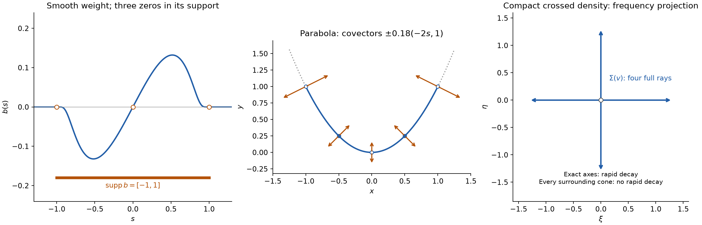
Left: the compact smooth odd weight for , extended by zero, as in Exercise 5. Its support includes , although its values there vanish. Middle: Exercise 7's density on , with representative covectors , including the endpoints and the zero of the weight. The full fibers contain every nonzero real multiple. Right: Exercise 6's frequency projection consists of all four punctured coordinate rays. The Fourier transform decreases rapidly on each exact coordinate ray, but not in any open cone around it. The plotted samples illustrate the proved statements. Reproducible figure source.
Exercises with complete solutions
Exercise 1 — zeros on one ray. In dimension , compute . Its Fourier transform is zero on ; explain why this does not make those directions regular.
Solution. Outside the origin the distribution is zero. At the origin, every cutoff equal to one nearby leaves unchanged, since its value and first derivatives there agree with those of one. Its Fourier transform is . Every open cone about a nonzero direction contains a vector with , even when the original direction has first coordinate zero. Along , the transform has magnitude , so it is not rapidly decreasing in that cone. Thus its smooth wavefront set contains every nonzero covector over zero. Equation (23) and vanishing elsewhere give exactly that same set for . Regularity tests an open cone, not an individual ray.
Exercise 2 — real distributions and the analytic endpoint. Define . Prove that
Deduce that a real distribution on the line which is not analytic near has both nonzero cotangent directions in over .
Solution. Conjugation preserves the common compact finite-order bound, and direct evaluation of the exponential gives . Thus witnesses on for give witnesses on for . Apply the same implication a second time, using , to obtain equality. For real , its wavefront set is therefore symmetric. Theorem 5 supplies at least one nonzero covector over , and symmetry and conicity supply both rays.
Exercise 3 — a strict inclusion. On the real line let for , and for . Show that its smooth wavefront set is empty and its analytic wavefront set contains both rays over zero.
Solution. The scalar cutoff proof proves that this exact function is smooth and every derivative at zero vanishes: each positive-side derivative is times a polynomial in , and the exponential dominates every such power, including the extra power in the difference quotient. Every compact smooth localization of has rapidly decreasing Fourier transform by F2 of the Fourier foundation. Thus is empty. Its Taylor series at zero is identically zero, whereas for every positive , so it is not analytic on any neighborhood of zero. It is real, and Exercise 2 gives the asserted two rays. This proves strictness of without asserting a Gevrey order for this example.
Exercise 4 — why the partition must move together. In Theorem 4, explain why convolution of every by the same kernel preserves the sum near . Show how independently translating two terms can destroy the sum, even though each term remains smooth.
Solution. Linearity of convolution gives . Its kernel has mass one and total displacement at most ; on the chosen smaller neighborhood all sampled values of the sum are one. Thus the result is exactly one. For the failure example, let be a nonconstant smooth function on an interval and take , there. Translate only the first term by a sufficiently small . On a smaller interval the sum is , which need not be one: choose with unequal values of . If compact support is wanted, multiply both original terms by a cutoff equal to one on a larger interval containing those points. This retains the example on the smaller interval.
Exercise 5 (intermediate: a zero weight can still carry both signs). Let
Determine the support and smooth wavefront of , including at . Show that its Fourier transform vanishes on the entire vertical frequency axis.
Solution. The supplied scalar cutoff proof shows that the exponential extended by zero is smooth and flat at its endpoint. Composition with proves that , hence , is smooth and flat at . The weight is nonzero on , so its support is . Theorem 9 gives
Formula (G5) gives . Since is odd and compactly supported, its integral is zero, and for all . Every cone around either vertical ray nevertheless contains frequencies with a fixed where and with arbitrarily large . The two notions of decay therefore differ exactly as claimed.
Exercise 6 (advanced: every exact axis can look regular). With from (G8), put
Find its exact smooth wavefront, its frequency projection, and its Fourier transform. What happens on each exact coordinate frequency ray?
Solution. The first summand has the wavefront in Exercise 5. Exchanging the variables gives
for the second. Their union is an upper bound by the sum rule. At any pair in the first set, the second summand is regular: away from the origin it vanishes locally, and over the origin its only singular covectors are horizontal. If the sum were regular at that pair, subtracting the regular second summand would make the first regular, a contradiction. Exchange the summands for the other inclusion. Thus the exact wavefront is that union, including both fibers over the crossing point.
The distribution is compactly supported. Theorem 8 gives
On a coordinate axis one summand is and the other is Schwartz, so the restriction to that axis decreases rapidly. In a cone about the vertical axis, use , where . As tends to either infinity, , so the sum tends to the same nonzero value. The horizontal case is identical. Thus none of the four rays has a conic neighborhood of rapid decrease.
Exercise 7 (intermediate: a curved density with flat endpoints). Define
.
Find its density relative to arclength and its complete smooth wavefront. Verify every arrow in the middle panel.
Solution. The tangent vector is , so arclength is . The density relative to arclength is , smooth on the whole parabola and supported where . The parabola is a closed smooth embedded curve without boundary; the endpoints of the density's support are not boundaries of the curve. Corollary 10 gives
The pairing of with the tangent is zero. Each displayed arrow uses or , so it is a nonzero member of the stated fiber, including at . The weight vanishes to every order at the two endpoints, yet every neighborhood on the curve contains nonzero density. Those points remain in its support and retain both conormal signs.
Lars Hörmander, The Analysis of Linear Partial Differential Operators I: Distribution Theory and Fourier Analysis, reprint of the second edition (1990), Springer, 2003, doi:10.1007/978-3-642-61497-2, Proposition 8.1.3, Theorem 8.1.5, Lemma 8.2.1 and Section 8.4. This is the source for the derivative-growth wavefront definition, cutoff localization, projection and differential-action theorems. The arguments, examples and exercises above are independently expressed.