Exposition by GPT-6 Astra (OpenAI), 4 October 2026. Public domain (CC0).
Adding two source locations explains both the power and the limitation of convolution. Two compact sources always give a distribution at their sums. Two unbounded sources do so when a bounded output can receive contributions only from a compact set of input pairs. This geometric condition will also control limits, associativity and local regularity.
Pairings are complex-linear, with no conjugation. We use U008, Proposition 1.2 and Theorem 5.1, for finite-order extensions and distributional limits; its formula (T1) characterizes bounded test families. The functional prerequisite, Sections 6 and 14.1–14.2, proves Baire's theorem and completeness of fixed-support test spaces. The scalar prerequisite, Sections 13.1–13.5 and 13.10, and the integration prerequisite, Sections 15.0–15.4, supply differentiation, compact cutoffs, ordinary integration and smooth approximation. All additional distribution constructions used below are proved here. The operator theorem also uses the exact Fourier inversion proof in the Schwartz prerequisite, F2–F4.
Pairings, parameters and tensor products
Write for an open subset of Euclidean space. For tests supported in a fixed compact set, write . A distribution is a linear form with a bound on each such space. A bounded test family has one common compact support and a uniform bound for every , by U008 (T1). Weak convergence means convergence on each test; strong convergence means uniform convergence on every bounded test family. The distinction concerns topologies even though U008 Theorem 5.1 proves that weakly convergent sequences also converge strongly.
B0. Localization and extended pairings. Define as the complement of the union of open sets where vanishes. It is closed, and whenever the compact support of misses it. Here is the localization step behind that assertion. Cover the compact support by finitely many open sets on which vanishes. Choose nonnegative smooth bumps supported in those sets with near the compact support, using smaller balls and the supplied cutoff construction. On that neighborhood divide by , and multiply by a compact cutoff supported there and equal to one near the test support. The smooth functions
are extended by zero outside the region where the denominator is positive. They sum to one near the test support. Thus , and every summand pairs to zero. The same partition proves that compatible local distributions glue: evaluate a test by the finite sum of its partitioned local pairings; a common refinement proves independence, and a fixed finite partition near each compact gives continuity.
If and is compact in , set
Two choices differ by a compact test whose support misses : at a point in their difference vanishes nearby, and at a point of the function vanishes nearby. B0 therefore proves independence. A common cutoff proves bilinearity whenever the finitely many relevant intersections are compact. Empty intersection gives zero. In particular a compactly supported distribution acts on every smooth function, with an estimate for one fixed cutoff. Multiplication by a smooth function and derivatives, defined by
are distributions by the finite product rule and have support contained in that of . A compactly supported distribution consequently has some finite global order. We denote the space of compactly supported distributions by .
A continuous function which defines the zero distribution is zero pointwise. Otherwise multiply its value at a nonzero point by a constant complex phase to make its real part positive; continuity and a nonnegative bump of positive integral in a small neighborhood contradict the zero pairing. This proves uniqueness when smooth local representatives are glued.
B1. Differentiating and integrating parameters. Suppose is smooth and, for in each compact parameter neighborhood, its -support lies in one compact subset of . Then
are smooth. Indeed a local order- bound for bounds the change in a pairing by the change in its test. For each , the fundamental theorem gives
Uniform continuity on a common compact gives convergence in that seminorm to the derivative, and the same estimate gives continuity of the derivative. Iterate. If has compact support, inserting one cutoff near it gives the statement without a support condition on .
If is compactly supported in both variables, a compact parameter integral can pass through :
To prove this, approximate the integral on a containing box by lattice Riemann sums. Every derivative in has uniform Riemann-sum error bounded by the box volume times its modulus of continuity in at the mesh diameter. The sums have a common compact -support. They therefore converge in every test seminorm. Apply the continuity of , and also the scalar Riemann-sum limit to the continuous function in (B2). The same proof works with finitely many continuous -derivatives when these control a finite-order pairing.
B2. Density of product tests and the tensor construction. Finite sums of are dense in , with approximating supports in a fixed compact product. To see this without a tensor theorem, extend a given by zero and form the ordinary integral
where both profiles are smooth, nonnegative, compactly supported and normalized. For small , the supports stay inside a fixed compact product in . Differentiating under the averaging integral shows
for every . Integration by parts in the ordinary compact integrals identifies these derivatives with derivatives of the kernels. For a fixed , Riemann sums in approximate (B4) in every , by the proof of B1, and each summand is a product test. Choose and then meshes so that the two errors in are at most . This gives one sequence converging in the test topology. The construction can keep supports in any prescribed product neighborhoods of the projections of .
For , , define
B1 gives a smooth inner test supported in the first projection of . If is supported in , and the two distributions have orders on those sets, then
This proves that it is a distribution. On a product test its value is . Reversing the pairings gives another distribution with those values; B2 proves equality and uniqueness. For three factors, apply B2 first to , and then to each test on . Products of three tests thus determine the distribution. Both associations and every permutation have the same values on them, proving tensor associativity and permutation symmetry. The support is exactly . Outside that product a small rectangle has one zero factor, so B2 and B0 give vanishing. At a point of the product, in every small rectangle each factor has a test with nonzero pairing, and their product has nonzero pairing. The derivative and separate multiplication identities follow either from (B5) and B1 or from their identical values on product tests.
B3. Tensor limits. Tensoring with a fixed distribution is separately weakly and strongly continuous. For weak continuity a fixed gives one fixed inner test by (B5). For strong continuity a bounded family of 's gives a bounded family of inner tests, by B1 and the local estimate for the fixed factor; its support stays in one compact projection.
If and weakly as sequences, U008 Theorem 5.1 supplies common finite orders and constants on any fixed compact projections. Thus (B6) bounds all tensor pairings uniformly in one finite seminorm. Approximate by B2 in that seminorm. On a fixed finite sum of products the pairings converge by ordinary scalar multiplication; the uniform bound controls the approximation error for every and the limit. Consequently
The strong conclusion follows from the weak conclusion and U008 Theorem 5.1 applied on the product open set.
Which pairs can contribute to an output
Define translation by
For a function this is ; for a point mass it gives .
For closed , addition is proper on the supports if
Equivalently, for every finite there is a finite such that
The sets are closed, so the equivalence is precisely the closed-and-bounded compactness criterion, applied to containing closed balls. A compact factor implies properness because . Properness implies that is closed: a convergent sequence of sums lies in one compact ball, so its contributing pairs have a convergent subsequence in .
Theorem 1.1 (convolution by addition). If , , and addition is proper on , define
The pairing uses B0. It defines a distribution with
Orders at most for the two factors give order at most . Also
Proof. The intersection of the tensor support with is closed and contained in the compact set . Hence B0 applies. For all tests supported in a fixed compact , choose one compact smooth on a neighborhood of . Then
Estimate (B6), the product rule and the chain rule bound this by a fixed finite seminorm of . When the factor orders are , no term differentiates more than times. Tensor symmetry proves commutativity. A test supported off has zero extended pairing, proving the support assertion.
For one derivative, apply to the compact test in (1.7). The term with vanishes near the tensor support wherever can be nonzero, because on a neighborhood of . Its pairing is zero by B0. The remaining term is , which is the pairing of . Derivatives do not enlarge supports, so the same properness hypothesis permits repetition and differentiation in either variable.
Evaluation at a point in (1.4) and then (1.6) give
Thus for every constant-coefficient differential operator ,
whenever the indicated supports sum properly.
There is also a maximal local output region. Let be the union of open balls such that is compact. For a compact , a finite such cover places , a closed set, inside a finite union of compact sets. Therefore (1.7) defines convolution on . A convergent sequence of sums with limit in eventually lies in one of these balls; compactness of its pairs proves relative closedness of . Consequently
Any open region where all compact output sets have compact preimages is contained in , by taking a small closed ball about each point. All preceding binary identities remain valid on this region.
Translating a distribution differentiates with a minus sign
Proposition 1.2 (strong translation derivatives). For every , the map is smooth in the strong distribution topology, and
Here smoothness means that all successive parameter difference quotients converge uniformly on each bounded test family, and that their limits are strongly continuous. In particular, for any fixed ,
The limit is two-sided and strong.
More precisely, fix compact sets of test supports and of translation parameters, and restrict . There are , independent of , such that, for every and integer ,
The same work for every .
Proof. All tests , with , , have supports in the fixed compact set
Choose a finite-order bound for tests supported there. For , repeated use of the fundamental theorem gives
For completeness, the case is the fundamental theorem after the substitution . Integration by parts in in the remainder, using
, expresses that remainder as
plus the next remainder. This proves the formula inductively for both signs of ; is immediate.
Apply (T7) also to every -derivative of order at most . The multinomial expansion, or repeated distributivity of , bounds each derivative of the remainder by
The integral is a smooth compactly supported test by the parameter argument B1. Distributional differentiation gives
Pairing the remainder with proves (T5).
For continuity under an arbitrary small displacement , the same fundamental-theorem argument on bounds the test difference in by , with one common support set for . On a bounded test family this tends uniformly to zero. Formula (T5) with , divided by , proves the first strong parameter derivative and its sign. Apply this argument successively to every distribution , and use the continuity just proved for those distributions, to obtain (T3). Finally (1.8) identifies , proving (T4). No compact-support assumption on is needed.
For a moving point mass, tends to . For the step function, tends to from either side: for it is the negative interval density , while for it is , also of mass .
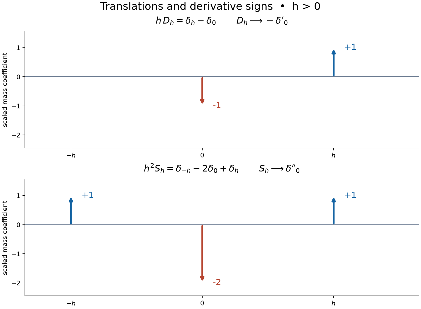
Figure. For , the arrows show the coefficients after multiplication by in the first panel and by in the second; they are point masses, not function values. Proposition 1.2 proves the first limit, and Solution 11 proves the second with its quadratic error bound. The Python figure source gives the exact coefficients and labels.
Smoothing and the exact derivative count
Theorem 2.1 (a regular factor). If and , their convolution is the smooth function
and
The map is continuous from to . If is compactly supported, it is also continuous from to , and from to .
For integers , an order-at-most- distribution convolved with gives a function by (2.1). If has compact support and order at most , the same holds for every .
Proof. On a compact output set , the tests in (2.1) have common support in . B1 proves smoothness and parameter derivatives. Differentiating in reverses the sign of differentiation in , which cancels the distributional derivative sign and proves (2.2). For compact , B0 inserts a fixed cutoff near its support and permits every smooth .
To identify the function with (1.4), pair it with a test . Formula (B3) and the translation substitution give
All needed cutoffs can be fixed near the compact contributing projections; B0 then removes them. For supported in a fixed compact , local order of on a compact neighborhood of gives
Every defining output seminorm therefore pulls back to an admissible input seminorm in U008's test topology. For compact , its fixed cutoff gives instead a seminorm of on a fixed compact neighborhood of , proving continuity. With fixed compact input support, (1.5) fixes a compact output support as well. The same estimates give continuity on each input support space into that output support space, and hence into by the defining inductive-limit topology.
For finite regularity use U008 Proposition 1.2 to pair with tests. The difference-quotient calculation in B1 converges in whenever the total number of parameter and test derivatives is at most . Uniform continuity of the derivatives of that last order gives continuity of the -th output derivatives. Thus (2.1) is . To justify (2.3) at this regularity, approximate in on a common compact neighborhood by smooth functions. The order bound proves convergence of the function pairings locally uniformly, while the smooth tensor pairings converge distributionally by (B5), or directly by their integral in . This proves agreement with (1.4). For noncompact and compact , apply the same approximation after a cutoff on the only compact region relevant to each output test.
Lemma 2.2 (Riemann sums with derivatives). For , ,
All sums and the limit have support in .
Proof. The sums are finite. For , compare the differentiated sum with the ordinary integral of on the cubes . The difference between each sampled integrand and its value at a point of that cube is at most
These are global moduli of continuity of the zero extensions, so the estimate is uniform in and tends to zero. Only cubes meeting a fixed bounded neighborhood of contribute; their total volume is bounded for small . This proves uniform convergence of every indicated derivative. Differentiating the ordinary integral is justified by the same uniform difference quotients. A nonzero summand requires and ; the integral vanishes off the same compact sum.
Ordinary convolution and the allocation of derivatives
Theorem 2.3 (finite regularity in both factors). If and , then the ordinary convolution is and
If in addition , then and
Either factor may be the compact one, with the corresponding exchange of their regularities.
Proof. On a compact neighborhood of an output point, all contributing 's in (C1) belong to one compact set , obtained by subtracting from that output neighborhood. The integral is absolutely convergent, bounded by . Uniform continuity of , followed by this bound, proves continuity. Difference quotients of through order converge uniformly on the fixed compact input region to the indicated derivatives, by the ordinary fundamental theorem of calculus. Their integrals therefore converge to the integrals of the derivatives. Induction proves (C1) as actual continuous derivatives.
Substitution gives the equal expression , proving commutation when the two expressions are defined. Apply (C1) first through order , and write its result as . Its integration is on the fixed compact support of . If , difference quotients through order converge uniformly on the compact set of relevant 's. Differentiating in proves (C2), with continuous right-hand side. For any multi-index of length at most , choose of length , and put . All derivatives through that total order exist by this argument, proving . Commutation proves the assertion when the other factor is compact. No boundedness of at infinity was used.
The ordinary integral gives the distributional convolution already constructed. For a compact test , all contributing pairs in
lie in one compact product, and the absolute integrand is bounded by a constant times . Fubini and the substitution prove (C3). B5 identifies this with the tensor pairing. When are both compact and continuous, Fubini on the full product also gives
For three continuous functions, at least two compact, Theorem 3.1 below gives ordinary associativity: every inner and outer convolution is a continuous function by (C1), their distributions agree by that theorem, and B0 identifies their continuous representatives pointwise.
Associativity and continuity need support control
Theorem 3.1 (associativity). Let be nonempty closed envelopes of the supports of . Suppose that the preimage of every compact set under addition of triples in is compact. Then both iterated convolutions exist and
Their common value on is the support-relative pairing of with . In particular, at least two compact factors suffice.
Proof. Fix . Pairs in with sum in a compact , together with third coordinate , lie in the compact triple preimage of . They form a closed subset, so pair addition is proper. Fixing a point of each other nonempty envelope gives the other pair properness statements. The sum is closed by Section 1. For a sequence whose sums lie in a compact set, choose . Triple properness gives a convergent subsequence of . Thus the pairs have a convergent subsequence; their relevant preimage is closed, so addition on is proper. This proves existence of both associations.
Here are the cutoffs that justify equality. Put . Choose a compact smooth cutoff equal to one near the preimage of in . In evaluating , the inner convolution involves only in the compact first projection of . Choose a compact cutoff near all pairs in with sums in that projection, using pair properness. Formula (1.7), B1 and the iterated tensor identity give the compact triple pairing
This test is compact: lies in , and in the second projection of . Its cutoff multiplier is one near every contributing point of the triple support with sum in . B0 identifies it with the canonical extended triple pairing. Repeating the same construction for the other association gives the same pairing, by B2's tensor associativity.
If two factors are compact, choose nonempty compact envelopes for them, using for a zero factor, and any nonempty closed envelope for the third. Bounded sums and bounded first two coordinates bound the third. Closedness then proves triple properness.
The nonempty-envelope hypothesis addresses an actual intermediate-existence issue. An empty envelope forces its distribution to be zero. The canonical triple pairing is then zero, and every association whose inner convolution is defined is also defined and zero. It does not define an otherwise missing inner convolution. For example, , , and have a proper empty triple preimage. The association is zero, whereas has no inner convolution under this construction, as (3.5) shows.
For , , , the theorem gives
Indeed both are compact distributions. Differentiation under the ordinary compact integral makes smooth. The left side is also a smooth function, by compact integration of the smooth against . The distributional identity therefore holds pointwise by B0. Lemma 2.2 justifies the interchanges even for merely continuous .
When at least one of has compact support, is uniquely characterized by
Associativity gives existence. For uniqueness, if a difference has for every test , apply this to the normalized shrinking profiles of Theorem 5.2. That theorem gives , so .
Theorem 3.2 (continuity with fixed support sets). On fixed closed where addition is proper, convolution is separately continuous in both the weak and strong distribution topologies. If , are weakly convergent sequences supported in , then weakly.
Proof. A limit has the designated support because every test in its complement has zero pairing with each term. For a fixed output test, use one cutoff in (1.7). Separate weak continuity is then B3. A bounded family of output tests has common compact support , so one such cutoff works for the whole family. Product and chain rules show that is bounded in the product test space. B3 proves separate strong continuity. Its joint sequence conclusion (B7), applied to each such fixed compact test, proves joint weak convergence.
The support constraint cannot be dropped:
The two inputs eventually miss each compact test support, but their sum stays at zero.
Proposition 3.3 (a cone algebra). If is a nonempty closed convex cone containing no nonzero line, distributions supported in form a commutative associative convolution algebra with identity .
Proof. For any fixed number of contributing coordinates, suppose their sums remain bounded while their maximum norm tends to infinity. Divide by and take a convergent subsequence in the product of closed unit balls. The limits lie in , have sum zero and include a vector of norm one. Its negative is the sum of the other limits, which also lies in . Closure under addition follows from convexity and positive scaling. Thus contains the line , a contradiction. All these additions are proper. Also by closedness and scaling, and . Theorems 1.1 and 3.1 give closure, commutativity, associativity and the identity. Bilinearity follows from a common cutoff in (1.7).
For , ordinary integration over gives
For the opposite half-lines and a nonnegative compact test positive near zero,
In fact for all sufficiently large a fixed-length interval of 's about contributes the same positive lower bound. Tonelli applies to this nonnegative integrand and proves divergence. Hence the ordinary positive pairing does not define .
Sequence limits on bounded output tests
Corollary 3.4 (strong sequence limits on proper supports). Suppose fixed closed satisfy
for every compact output . If , weakly with supports in these sets, then
The same conclusion holds in if compactness in (3.4a) is required only for .
Proof. The support of each limit lies in its closed envelope. For a bounded output test family , let contain all its supports and choose near . The family
is bounded by the product and chain rules. Put . Formula (1.7) gives
by B3. If , the zero cutoff gives zero directly. This proof uses only compact output subsets of , so proves the local version too.
Local smoothness can come from either factor
Theorem 4.1 (finite regularity at an output point). Let , , and an integer . Suppose that every has a neighborhood and an integer such that either
or
Then is near .
Proof. Shrink the neighborhoods and use compactness of and the explicit partition construction in B0 to write
Choose , equal to one on a neighborhood of . These are compact subsets of the indicated open sets. A single sufficiently small neighborhood of satisfies
The support of cannot add to a point of with the support of . Theorem 1.1 therefore gives on . In (4.1) the first factor is compact of order at most and the second is compact ; in (4.2) the roles reverse. Multiplication by a fixed smooth cutoff preserves the claimed order by the product rule. Theorem 2.1 makes each term . Their finite sum proves the result.
Corollary 4.2 (singular support). With compactly supported,
Here the singular support is the closed complement of the set where a distribution is represented by a smooth function.
Proof. The right side is closed because its second factor is compact: a convergent sequence of sums has a convergent subsequence of second coordinates, and hence of first coordinates. If misses this sum, every has either a neighborhood where is smooth or one whose reflection about is a smooth region for . Shrink it so the other distribution has a finite local order. Choose this finite cover and the cutoffs of Theorem 4.1 once, independently of . The selected smooth factor has every derivative, and the other factor has its fixed finite order. Thus the same finite sum on the same neighborhood is for every ; it is smooth there. B0 ensures agreement of these representatives.
Ordinary support inclusion can be strict. For
the two contributions at cancel. The input-support sum is , and the output support is .
Corollary 4.3 (singular support on the proper output domain). For closed support envelopes and the maximal local properness region of Section 1,
The sum on the right is relatively closed in .
Proof. A convergent sequence of sums of singular points, with limit in , eventually lies in a compact ball inside . The contributing pairs then have a convergent subsequence. Closedness of both singular supports gives the relative closedness assertion. Fix outside that sum and a ball about it with compact closure . Take compact cutoffs equal to one near the two projections of . Formula (1.7) gives
Multiplication by a smooth cutoff introduces no singularity. Corollary 4.2 therefore places the singular support of the right side in the sum of two compact subsets of the original singular supports. That compact sum misses , so the right side is smooth near . This proves (4.7). Empty factors give the zero distribution and cause no exception.
Smoothing inside an arbitrary open set
Proposition 5.1 (the local convolution domain). For open , , and compactly supported with , convolution is canonically defined on
It depends only on near at an output point . Derivatives transfer as in (1.6), and
For , it is the smooth function .
Proof. If , take and the convolution zero. Otherwise, for , the compact set has a positive distance from the closed complement, unless that complement is empty. Its sufficiently small translates stay in , proving that is open. For compact , the continuous image of is compact and contained in . The contributing part of the tensor support in is contained in . B0 and (B6) consequently define its pairing with by fixed compact cutoffs. They prove continuity, independence of cutoffs and local dependence; the derivative argument of Theorem 1.1 is unchanged.
The set in (5.2) is relatively closed. For , a subsequence has , so . Relative closedness of includes this limit. Tests off the sum have zero pairing, proving (5.2). B1 and the calculation (2.3), with the same local cutoffs, prove the smooth formula.
Theorem 5.2 (shrinking smooth averages). Suppose smooth compact profiles satisfy
For every , the locally defined converge strongly on tests in to . In particular any family of nonnegative normalized shrinking profiles works, without requiring one fixed shape.
Proof. Every fixed compact test support lies in the output domain for small enough . Formula (B5), a translation substitution, and (B3) give
The averaged tests have support in , hence in one compact subset of for small radii. Subtract using the normalization. The fundamental theorem on the segment from to gives
Use the finite-order bound of on that compact neighborhood. On a bounded family of 's, has a common bound, so the pairings tend uniformly to zero. This is exactly the stated local strong convergence. For nonnegative normalized profiles the norm is one.
Corollary 5.3 (compact smooth approximation). Every distribution on an open is a strong distribution limit of a sequence in .
Proof. Use the compact exhaustion supplied by the integration prerequisite, and cutoffs near , compactly supported in . Multiplication followed by zero extension makes a compact distribution on : explicitly it acts on as . Choose nonnegative normalized profiles with support radius
omitting the second bound if ; a zero cutoff requires no distance restriction. Put . Theorems 1.1 and 2.1 put in . On a fixed compact test support and its one small compact neighborhood, eventually. Formula (5.4) therefore makes its pairing with exactly its pairing with the local . Theorem 5.2 proves convergence uniformly on every bounded test family. If , the only distribution is zero and the zero sequence suffices.
Norm convergence of varying averaging kernels
Theorem 5.4 (uniform, integral and local approximation). Let the smooth compact kernels satisfy (5.3), and put . For , , the convolutions are smooth and
For , they converge to uniformly with every derivative through order , and their supports eventually lie in one common compact set. For an open , the corresponding statements hold locally on every compact subset of for and data, on the output domains of Proposition 5.1.
Proof. Translation continuity in , including , is proved in the supplied measure foundation, Section 15.3. It uses density and is valid for every finite . Normalization gives, for almost every ,
For , Hölder applied with measure , followed by Tonelli, gives
For , the triangle inequality and Tonelli give the same formula with exponent zero. These bounds also justify the almost-everywhere integrals. Since the kernel is supported in the radius ball, (C6) implies (C5), and translation continuity makes the supremum tend to zero. An function is locally integrable by Hölder on compact sets. Theorem 2.3 with the compact smooth kernel, for every , proves smoothness of its convolution representative.
For , Theorem 2.3 allows the derivative to fall on . Each , , is uniformly continuous on the whole space: it is continuous and zero outside a compact set, and uniform continuity on a slightly larger compact neighborhood handles its boundary as well. Thus
For , all supports lie in
, which is compact.
For the local statements, fix and choose such that . The compact cutoff construction in Local data and compatible products gives , equal to one near that compact neighborhood. The product , extended by zero, belongs to global , or to for data. For , its convolution equals the local convolution on a neighborhood of , since all input points there lie where . The global estimates now imply the required local norms or uniform derivative estimates on . This localization needs no extension or growth assumption on the original data outside .
Corollary 5.5 (locally integrable functions are determined almost everywhere). If have equal integrals against every test in , then almost everywhere on .
Proof. Put . Choose nonnegative normalized compact smooth kernels with radii tending to zero. For in a fixed compact and a sufficiently small radius, is a test in . Its pairing with is zero by hypothesis. Thus on . The local conclusion of Theorem 5.4 yields . Exhaust by countably many compact subsets; the union of the corresponding null sets is null. This proves the assertion. If both functions are continuous, they agree everywhere by B0, or because a nonzero continuous difference would have nonzero magnitude on a ball of positive measure.
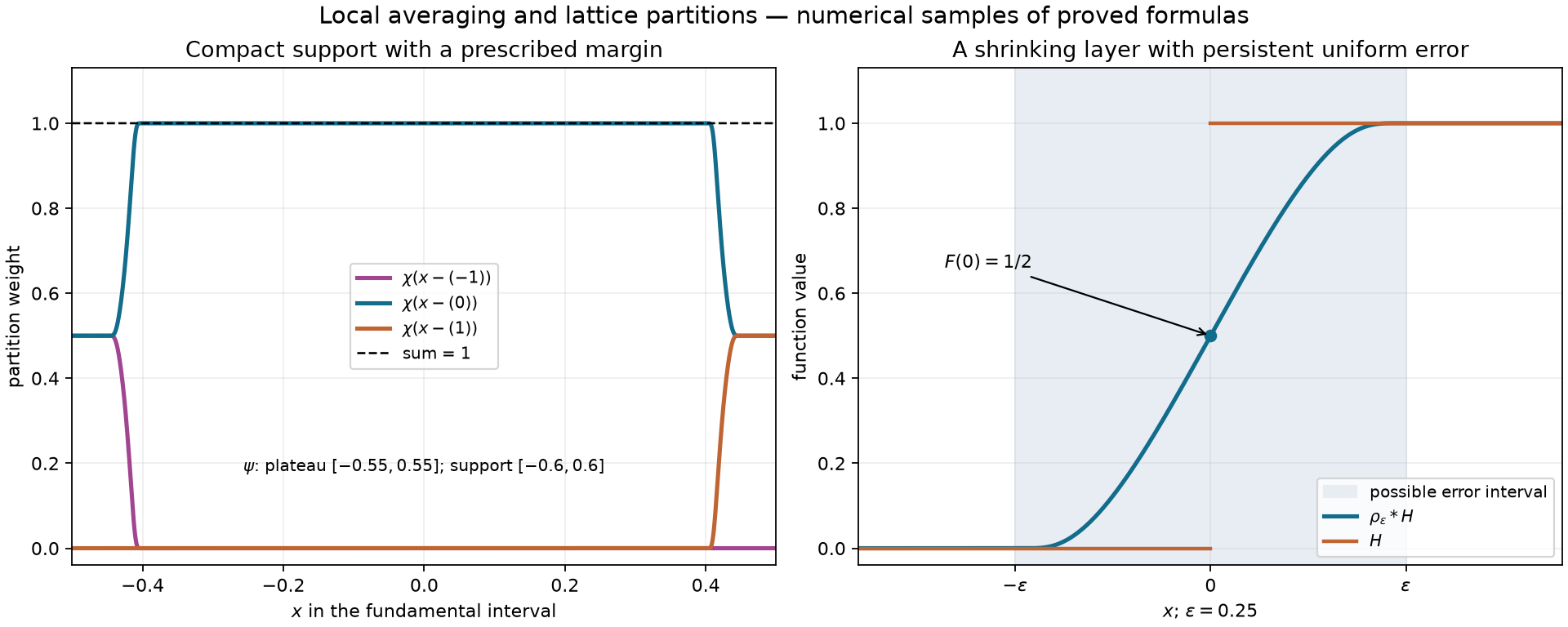
The finite- restriction is essential: smooth averages of a step converge in each local finite- norm but retain an essential supremum error of , as Solution 13 proves.
The right panel uses the even normalized kernel proportional to on , zero elsewhere, and . The averaged step equals the step outside . Its error is at most , with that essential supremum attained as a limit near zero. The left panel illustrates the lattice normalization in Local data and compatible products, Proposition 1.2. Curves are numerical samples; (C5)–(C7) and Solution 13 give the proofs. Reproducible figure.
Finite measurements and the weak topology
A basic weak neighborhood of specifies finitely many tests and positive tolerances , and consists of the distributions satisfying
Pairings remain complex linear. The empty list imposes no condition.
Proposition 5.6 (the continuous dual of the weak distribution space). A complex-linear map is continuous for the weak topology if and only if there is a unique such that
Proof. Evaluation on a fixed test is continuous by (W1). Conversely, continuity at zero supplies a basic neighborhood on which . Define the linear map
If , every scalar multiple of is in that neighborhood. Linearity and the bound force . Thus induces a well-defined linear functional on the subspace . Choose a basis of that subspace, extend it to a basis of , and extend by assigning zero to the additional basis vectors. This finite basis construction terminates after at most independent choices. In coordinate form the extension is . Hence gives (W2). If the list is empty, the same scaling argument gives and we take .
For uniqueness, the point mass is a distribution for every , since . Two representing tests therefore have equal values at every . If is empty all the spaces are zero and the conclusion still holds.
Proposition 5.7 (exact interpolation of finitely many measurements). Given and finitely many , there is with
The support of can be contained in the union of the test supports. Consequently the distributions defined by compact smooth functions are weakly dense in .
Proof. Choose a basis from the finite span of the . For , take . Otherwise define
All these integrals are over one compact set. The Hermitian matrix is positive definite: for ,
Independence makes the smooth function inside the modulus nonzero somewhere; continuity gives a ball where its squared modulus has a positive lower bound. That ball has positive volume. If , (W6) would force . Thus the columns are independent and form a basis of , so has a unique solution. This uses only finite-dimensional basis extension, not an infinite-dimensional representation theorem.
Formula (W5) gives a compact smooth , supported in the union of the supports, and . Every original test is a linear combination of this basis, so (W4) follows. The basis may be selected from the original tests, giving the asserted support inclusion. Every neighborhood (W1) consequently contains a regular distribution with exactly the same listed values as . This proves weak density. Corollary 5.3 supplies the stronger sequential approximation with control of all bounded test families.
The conjugates in (W5) are essential: the distributional pairing is bilinear, while the positive Gram matrix uses a conjugate to guarantee invertibility. Exact agreement on a finite list also does not identify the full distribution. Solution 15 exhibits a test on which the interpolant and its target disagree.
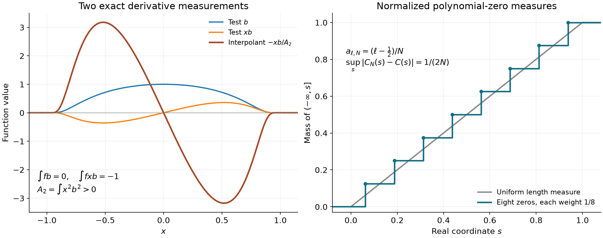
Figure. Left: the exact interpolant for the two tests and target , where for , zero otherwise, and . The plot evaluates this positive normalization by numerical quadrature; the identities and follow exactly from parity and the definition of , as in Solution 15. Right: the cumulative masses of eight atoms of weight at and of uniform length measure on . Their maximum cumulative difference is . These atoms are the normalized logarithmic curvature of the polynomial in Compactness and complex-line positivity, Solution 9. Editable figure script.
Translation-invariant operators have one convolution kernel
We first prove the two kernel facts needed for the operator theorem.
K1. Constructing a kernel from a separately continuous pairing. Suppose is a complex bilinear form on which is continuous in each variable with the other fixed. There is a unique satisfying .
Fix compact supports . On the complete metric space , form the closed sets
They are closed because is continuous for each . Their union is the space: continuity of gives one finite-order bound for each fixed , and increasing bounds its order and constant. The complete-space and Baire proofs are in the functional prerequisite, Sections 6 and 14.1–14.2. Thus some contains . Subtract the inequality at from that at , and then rescale . Since includes the zeroth derivative, it is zero only for the zero test. This gives
Specifically works. This is the joint estimate we need; separate continuity alone was the hypothesis.
Choose compact smooth cutoffs equal to one on neighborhoods of two given closed boxes, and apply (K1) with their supports. Put . The Schwartz prerequisite F2–F4 proves the Fourier convention and inversion
Define
The second factor depends continuously on the frequencies: the compact exponential tests depend continuously on them in every derivative seminorm, and (K1) controls the change in either argument of . This is an absolutely convergent scalar integral. Indeed (K1) bounds that factor by . For on any fixed compact support, integration by parts from F2 gives
Choose . The product of these bounds is integrable: on its integral is bounded by a constant times , whose sum is geometric, and the unit ball has finite volume. Thus has a finite test seminorm bound and is a distribution.
For , Fubini gives . Fourier inversion and (K1) show
To justify the passage through , truncate the frequency integrals to boxes and approximate by Riemann sums. Every derivative of grows at most polynomially in ; the rapid decrease of bounds the tails in every test seminorm on the one fixed support . The same holds for . The truncated sums therefore converge in the fixed-support test spaces, and the bound (K1) permits both limits. This proves (K4) without a vector-valued integration theorem.
On tests supported inside the boxes where both cutoffs are one, this distribution is independent of the cutoffs: by B2 approximate such a test by finite product sums supported within those boxes, and use (K4) for each sum. Choose increasing boxes exhausting each Euclidean space. The resulting distributions agree on the smaller product boxes by this argument. For an arbitrary compact test choose one containing product box and use its functional; agreement proves independence and linearity, while its finite bound proves continuity. This constructs . Product-test density B2 proves uniqueness. No growth condition on outside fixed compact supports has been imposed.
K2. A distribution constant in a whole group of variables. If has for every , there is a unique with .
Choose one-dimensional normalized compact smooth profiles , and write . For a test , integrate first in , obtaining . The difference has integral zero in , so
is a compact smooth test with . Smoothness follows from ordinary differentiation under the compact integral. It vanishes below the containing interval of the two supports and above that interval by zero total integral; the other supports lie in fixed compact projections. Repeat the same construction for in , then in every subsequent coordinate. Multiplying the new primitives by the previous profiles gives compact smooth tests with
Define . The product estimate for tests makes a distribution. Applying to (K5) kills every derivative and gives , precisely by B5. Testing with also proves uniqueness.
Theorem 6.1 (translation invariance). Let
be a linear weakly continuous map with for every . There is a unique such that
Every output is smooth, and is continuous.
The conclusion also holds for a linear translation-commuting map which sends every sequence tending to zero in to a sequence tending uniformly to zero on compact output sets.
Proof. The bilinear form is separately continuous: one direction is the output being a distribution, and the other is weak continuity of . K1 gives
Translation commutation implies
By B2 this invariance holds for every test on the product. The invertible linear coordinates have absolute determinant one. Define
Composition with this linear map preserves compact supports and bounds each derivative by a finite sum of derivatives, so is a distribution. Simultaneous translation of is translation of alone. Equation (6.4) consequently gives . Difference quotients in converge in the test topology by the fundamental theorem, with one common compact support for small . Hence every is zero. K2 gives .
The test is compactly supported: lies in and lies in . Thus B5 and (2.3) give
Theorem 2.1 proves the smoothness and continuity into . After that conclusion, recover directly by
This proves uniqueness as well.
For the variant, regard each continuous output as a distribution. For a fixed output test , the linear form sends test sequences tending to zero to zero, by the uniform convergence on and the bound . U008 Proposition 1.1 makes it a continuous test functional. Thus is weakly continuous into , and the first part applies. The original continuous output equals the smooth representative pointwise by B0.
The geometry is that simultaneous translation fixes only the difference . The construction places no polynomial growth condition on ; Fourier inversion in K1 was used only for compact tests.
Exercises
Cancellation and derivative signs. For , on the line, find , , their test pairings and the input and output supports.
Causal integration and a delayed jump. With , , compute and , justifying associativity despite the noncompact factors.
Normalization without a norm bound. Let be even, nonnegative and normalized. Put and . Find its integral, supports and distribution limit, and identify which hypothesis of Theorem 5.2 fails.
The finite-regularity threshold. Extend for by zero. Prove that is but not , and identify in Theorem 2.1.
A shifted output domain. Let , , . Find the domain in Proposition 5.1, the test pairing and the singular support of .
Reflection and translation. Show that is continuous on tests but is not convolution with one distribution. Use both translation commutation and the recovery formula (6.7).
Properness from geometry. For , bound each coordinate of any finite contributing tuple whose sum lies in a ball of radius . Explain the obstruction for a closed convex cone containing a nonzero line.
Translation invariance and locality. If satisfies Theorem 6.1 and for every test, prove that is a finite constant-coefficient differential operator. Prove the converse.
Jets and tails on a half-line. For , , compute the convolutions and their strong limit. Give one fixed proper pair of support sets and a direct bounded-test proof.
A curved proper pair. Let , , . Prove properness of addition on , and compute the strong limit of
including all translated derivatives.
Centered translation differences. For arbitrary and , find the strong limit of , and give an error of order on each bounded test family. Calculate both signs explicitly for and in one dimension with .
Sharing three derivatives — intermediate. For , , express without asking either input for a third derivative. Justify continuity and compactness of the relevant integration domain.
A persistent uniform error — intermediate. Let be even, nonnegative and normalized, with support in . For and , prove that the error is supported in , has essential supremum , and satisfies for every compact and finite . Explain why this is a local example, since .
Zero mass with a nonzero convolution — intermediate. Let have integral one. For and , compute the integral and first moment of . Deduce that its vanishing integral does not make the convolution zero.
A derivative measured twice — intermediate. Let be the even compact smooth bump in the figure, and put . For the tests and target , find the interpolant in Proposition 5.7. Show that it fails to match the same target on the test .
Complex tests and the conjugation — intermediate. Replace the tests in Exercise 15 by . Compute their Gram matrix, target values and interpolant. Show explicitly that omitting the conjugates from (W5), while retaining the same coefficients, gives the wrong second measurement.
Freedom inside any open region — advanced. Fix finitely many tests on an open , . For every nonempty open , construct a nonzero whose pairings with all the listed tests vanish. Deduce nonuniqueness of smooth interpolation even when the permitted perturbation region is prescribed.
Complete solutions
Solution 1. Evaluation and (1.8) give
Their pairings are and . Each input has support , so their support sum is ; the nonzero output masses are precisely at . Smooth tests supported near either point show that neither is removable from the support.
Solution 2. Every support lies in the pointed closed cone , so Proposition 3.3 supplies associativity. The fundamental theorem gives
Thus , and
Both pair as ; endpoint values of the indicator have no effect on its distribution.
Solution 3. The derivative of a compact smooth function has integral zero. Hence , and its support lies in . Integration by parts and scaling give
The limit is , by compact uniform convergence of the two test factors. But
Here , since a nonzero normalized compact function is not constant. The uniform bound in (5.3) fails. Taking shows directly why the remaining hypotheses do not suffice.
Solution 4. At an endpoint let be the inward distance. Then on the inside and zero on the outside. Derivatives through order three match at the endpoint; the fourth has inside limit and outside limit zero. Thus , while . The order-at-most-two pairing of is , so Theorem 2.1 with applies and gives
Near an endpoint this is on the inside. Its second derivative consequently has inside limit and outside limit zero. It is and not . The two-derivative order is exact: with a compact satisfying , the tests have norm tending to zero but constant nonzero second derivative at zero.
Solution 5. The principal value on exists directly because
The fundamental theorem proves the bound and integrability at zero. This is the symmetric punctured-integral limit, and away from zero it is the function . It cannot be smooth near zero, because uniqueness of continuous representatives on either punctured side would make such a smooth representative equal to the unbounded .
Now means . The convolution is the translated principal value there, with singular support exactly . Its pairing is
The translated test is compactly supported inside , so no extension of outside is used.
Solution 6. Reflection takes one fixed compact support to its reflection and preserves every derivative supremum, up to irrelevant signs. It is therefore continuous on . However ; for , a small bump whose two translated centers differ shows this is not . Every convolution operator commutes with translations: (2.1) gives . Hence reflection is not convolution. Independently, (6.7) would give , so , whose convolution operator is the identity. Reflection changes the sign of a nonzero odd test, giving a contradiction.
Solution 7. For a contributing tuple , every . The sum being in a radius- ball implies , hence
The contributing tuples over a compact output set are closed and bounded, so compact. If a cone contains for a unit vector , the pairs have sum zero and unbounded coordinates. More concretely the two positive distributions and are locally finite, but their proposed positive convolution pairs to infinity with any nonnegative test positive at zero: each matching pair contributes its positive value at zero. This establishes an obstruction for that pair, without asserting that every pair supported in such a cone fails.
Solution 8. By (6.7), a test supported away from zero satisfies , because locality keeps the smooth output supported away from zero. Hence . The complete point-support proof in the angular prerequisite, A3, gives
That proof uses a shrinking cutoff, the finite-order estimate and the Taylor remainder to annihilate tests with zero -jet; it then supplies the coefficients and their uniqueness. Substituting into (1.8) gives . Conversely every such finite operator is continuous on each test support space by its derivative estimate and hence on ; it commutes with translations and its derivatives vanish wherever the input vanishes locally. It is therefore local and satisfies the hypotheses of Theorem 6.1.
Solution 9. Choose . A compact output bound bounds both between zero and , proving properness. The input weak limits are , since the masses at eventually miss every compact test. Bilinearity, translation and derivative transfer give
For a bounded family supported in , all three nonorigin terms vanish exactly once : the tests, including their derivatives, are zero in neighborhoods of those points. The strong limit is thus , pairing as , in agreement with Corollary 3.4.
Solution 10. The parabola is closed. If a compact output set has second coordinate bounded above by , a contributing pair of parameters satisfies . Either there are no such pairs or . Closedness and this bound prove properness. The supports of both input sequences lie in , including the derivative at the origin. Their weak limits are . Expanding gives
All three nonorigin locations escape every compact set. On any one bounded output test family their point and derivative pairings therefore vanish exactly for large . The strong limit is , pairing as . Both this direct argument and Corollary 3.4 allow these noncompact fixed support envelopes.
Solution 11. Use (T5) with at the displacements and . The constant and odd terms cancel in the sum after subtracting . The quadratic terms sum to . The sum of the two remainders is bounded, on a fixed test support, by . Thus
Every bounded test family has a uniform bound for this seminorm, proving strong convergence and the asserted rate. In one dimension with , the pairing is
, the pairing of . With , the limit is , whose pairing is . These signs follow from differentiating the distribution; the displayed second-difference coefficients are .
Solution 12. Take , in (C2). Then
The -integral is on . On any compact output neighborhood, lies in one compact set where the second derivative of is continuous and uniformly continuous. The integral is therefore continuous in . Theorem 2.3 proves it is the actual third derivative; the first factor supplies one derivative and the second supplies two.
Solution 13. Substitution gives
The function is zero for , one for , and satisfies by evenness. It is nondecreasing, with . Thus the error vanishes outside the stated interval and its magnitude is at most . Continuity of at zero makes the error arbitrarily close to on sets of positive measure on either side of zero, so the essential supremum is exactly . Integrating the pointwise -th power bound over a set of length at most proves the local estimate. The global theorem does not apply to , but its local form does. The error itself does belong to global and satisfies the same bound there.
Solution 14. Integration by parts gives and ; boundary terms vanish by compact support. Formula (C4) gives . Fubini and , justified on the compact input product, yield
Consequently is nonzero. Cancellation of total mass is compatible with a nonzero first moment and nonzero function.
Solution 15. The bump is smooth at both endpoints by the exponential flatness construction in the scalar cutoff foundation. It is positive on , , and by evenness. Hence the target values are . Parity makes the Gram matrix diagonal with entries and . Formula (W5) gives . Its two pairings are . However,
The numerator is positive on a nonempty interval away from zero. Thus the finite measurements agree while the distributions differ.
Solution 16. The mixed Gram entries are and , both zero. The diagonal remains ; the target vector is . Thus , , and
Using instead gives , whose second pairing is , not .
Solution 17. If there are tests, choose disjoint closed balls of positive radius inside . This is possible by placing finitely many distinct points in a small ball contained in , and then choosing radii smaller than their mutual distances and distances to that ball's boundary. Let be a nonzero smooth bump in the -th ball. Form the -by- matrix . Its columns are linearly dependent in , so some nonzero vector satisfies . Then has the required pairings and support. It is nonzero because the supports are disjoint and one coefficient is nonzero. Adding any scalar multiple of to an interpolant preserves every listed measurement.
Programme proof locations and sources
U008, Order, positivity and distributional limits: the definition and bounded-family characterization (T1), Proposition 1.2 for finite differentiability, Proposition 1.1 for the sequential criterion, and the entire proof of Theorem 5.1 for uniform order and strong sequential convergence.
Functional prerequisite, Sections 6 and 14.1–14.2: the complete Baire and test-space completeness proofs used in K1. Scalar prerequisite, Sections 13.1–13.5 and 13.10, and integration prerequisite, Sections 15.0–15.4: scalar differentiation, compact cutoffs, integration, translation changes and smooth approximation.
Schwartz prerequisite, F2–F4: the seminorm estimates, integration by parts and two inverse identities used in (K2)–(K4). Angular prerequisite, A3: the full finite point-jet proof used in Solution 8.
Semyon Dyatlov, Lecture notes for 18.155: distributions, elliptic regularity, and applications to PDEs, freely accessible MIT notes, 2 October 2026 version. Propositions 6.3 and Lemma 6.8 provide the parameter and integral arguments; Theorems 6.4, 6.7, 6.10 and 7.1 provide smooth convolution, approximation and tensor construction. Chapter 8 gives the proper-support pairing and singular-support localization. The Fourier kernel sketch in Theorem 7.6 is expanded here into the complete compact-cutoff construction K1, with its norm bound, convergence and compatibility proofs.
Richard Melrose, 18.155 Lecture 15: Schwartz's kernel theorem, freely accessible MIT lecture, 1 November 2016. Pages 2–4 explain separate continuity, the Baire estimate and localization by cutoffs. The kernel construction here uses the supplied Fourier inversion proof and the explicit integral (K2); it does not require the lecture's additional Sobolev-space machinery.
Lars Hörmander, The Analysis of Linear Partial Differential Operators I: Distribution Theory and Fourier Analysis, second edition, Springer, 2003, §1.2, pp. 14–15, for tests and determination of locally integrable functions; §1.3, pp. 16–18, for ordinary convolution, allocation of derivatives and approximation; §4.2, Exercise 4.2.5. ISBN 978-3-642-61497-2. Proposition 1.2 proves the translation limit and its bounded-test remainder estimate.
The ordinary convolution identities (C1)–(C4), norm estimates (C5)–(C7) and almost-everywhere determination are proved in Theorems 2.3 and 5.4 and Corollary 5.5. The local cutoff used in Theorem 5.4 is constructed in Local data and compatible products.
Lars Hörmander, The Analysis of Linear Partial Differential Operators I: Distribution Theory and Fourier Analysis, reprint of the second edition, Springer, 2003, doi:10.1007/978-3-642-61497-2, §4.1, pp.88–100: smooth approximation, weak duality, subharmonic limits and logarithmic curvature. The finite-measurement and integer-weight constructions above provide their full arguments.