Analytic equations and characteristic directions

An analytic differential equation determines every noncharacteristic singular direction of its solution from the corresponding direction of its right-hand side. The estimate holds for the analytic wavefront set and for every derivative-growth scale considered here. Its support consequences are stronger than ellipticity: Poisson brackets can rule out the end of a solution's support even when characteristic covectors remain.

We use Derivative growth and finite-order localization, especially its analytic derivative bounds, controlled cutoffs and bounded-distribution criterion; Cones and derivative-growth wavefronts, Theorems 3–4 and 7; Both analytic directions at support boundaries, Theorem 1, Corollary 2 and Proposition 3; and Characteristic motion and closed-set barriers, Corollary 5. Fourier inversion and finite-order pairings have their proofs in the supplied Fourier foundation, F1–F5, and convolution lesson, B0–B2. The calculus and integration foundations supply compactness, Leibniz' rule, convergent power series and the integrals below.

1. Symbols, directions and finite derivative budgets

Let be open, . Our coefficients may be complex. Write

The characteristic set is . A noncharacteristic pair has . A derivative-growth sequence satisfies

By definition, when bounded compact distributions , equal to on one neighborhood of , satisfy in one cone about . Boundedness entails one compact support, one finite distributional order, and uniform constants. We keep this requirement when changing the index of a cutoff.

Here is the estimate that prevents a repeated analytic differentiation from losing an extra factorial. Fix a compact , and a family of smooth coefficients satisfying uniformly

For , , define a finite seminorm

Lemma 1 (spending a derivative budget). Multiplication by any coefficient in (3) has norm at most in (4). Also

Consequently a product of analytic multiplications and derivatives is bounded by multiplying these constants, provided the remaining derivative budget is reduced after each differentiation. The order of the factors is retained.

Proof. For , the product rule, grouped by , gives

The identity is the coefficient of in . We used . Formula (5) follows by retaining the derivative in the original maximum. Applying these two inequalities from the rightmost factor to the left proves the last assertion.

Analytic coefficients satisfy (3) on compact neighborhoods, by the analytic derivative criterion in the prerequisite lesson. We also need reciprocals uniformly in a frequency direction. Suppose is a finite linear combination of analytic -functions with bounded continuous coefficients in , where ranges over a compact set, and near . The Taylor coefficients about any have a common absolute majorant , after dividing by . Indeed (3), divided by the multi-index factorial, and , give that majorant. Choose a common making its value at at most . The geometric series for the reciprocal converges absolutely there, with absolute coefficient sum at most . Thus

The series equals the ordinary reciprocal by its finite geometric identity and convergence. It therefore supplies its actual derivatives. Products and any fixed number of derivatives of these coefficients again satisfy (3): Leibniz' rule and , for fixed , prove this after enlarging constants. The latter inequality follows from , with the fixed polynomial bounded by an exponential. This proves all uniform reciprocal estimates used below.

2. Compact amplitudes with an exponential prefactor

The cutoffs used to construct a bounded distribution sequence have uniform fixed-order bounds. The auxiliary amplitudes used inside a transpose identity need a different estimate, permitting an exponential prefactor.

Lemma 2 (an amplitude estimate on a smaller cone). Suppose is compact, is a closed frequency cone, and . Let have order at most on a neighborhood of . Suppose is supported in and

All constants are independent of the auxiliary parameter . For , set . Then, uniformly in that parameter,

In particular may be the frequency at which the transform is evaluated.

Proof. We may discard empty base or angular sets. Closedness of the wavefront set and compactness of give a compact neighborhood of and a slightly larger open cone containing in its angular interior, with all pairs over and the angular closure of still regular. To justify a uniform enlargement, otherwise a sequence of nonregular pairs at distances tending to zero from that compact product would converge to a nonregular pair in the product. Shrink inside the neighborhood where the order bound holds.

Use the controlled cutoffs of the prerequisite lesson supported in , equal to one on a fixed neighborhood of . Compact localization from the wavefront lesson produces equal to there, with

The first bound has order , because multiplication by those cutoffs has uniformly bounded derivatives at every fixed order.

Integration by parts up to order in a coordinate with largest frequency component, and the zero-order bound in (8), give

Explicitly the two estimates are and . Their minimum is at most . The fixed support volume and the factor are absorbed into . For , (11) has integral at most : scale , bound the integral of by that of , and absorb into an exponential. The integrability follows by the dyadic annulus argument already proved in the wavefront lesson.

The exact Fourier pairing is

It follows from Fourier inversion of the smooth compact factor inside the finite-order pairing, with convergence in the necessary finite smooth seminorms; this is the full identity proved in the wavefront lesson, Theorem 3. For each fixed , smooth compact support makes the integral absolutely convergent.

Put . On , the second estimate in (10), together with the integral bound for (11), gives . On the complement, angular separation or gives . The other part of (10) and (11) therefore bound the remaining integral by

For the last step scale , use , and dominate by . Its integral is uniformly bounded for the integers . Since , the elementary fixed-shift estimate finishes (9). For clarity, divide the first expression by : , and the remaining fixed power of is bounded by an exponential. Every bound was uniform in .

3. A finite transpose construction

Fix a compact neighborhood and a closed cone on which for . Assume . Their neighborhoods can be chosen slightly larger with the same property. Homogeneity and the compact unit-frequency slice give . Choose real controlled cutoffs , supported in , equal to one on a fixed smaller neighborhood. For every fixed ,

We use the bilinear distribution transpose, without complex conjugation: . The exact product rule gives

Indeed . With , the terms sum to . Group the remaining terms by , and define

These have differential order at most . After expansion they are times a finite sum of analytic coefficients depending on , followed by derivatives of order at most . All coefficients obey common bounds (3), by (7) applied to . Thus the identity is , where .

For , let . Sum every ordered word of total degree at most , including the empty word:

Each lies in . Left multiplication by prepends one letter. Every nonempty word of degree at most cancels once; the remaining first-crossing words are precisely the second line. Therefore

Every error word has total degree with . The total number of words of positive degree at most is at most : compositions of into positive integers correspond to choices of cuts in its gaps and number ; restricting each part to at most can only reduce the count.

Here are the uniform estimates, including the derivatives needed for distributional pairings:

To prove them, choose in (4) also large enough that (14) with gives . The finite coefficient expansion of , Lemma 1, and , give . Apply this successively, reducing the budget by each actual degree. Since , its factors , the factors , and , give the first line. For the second line each word has , leaving at least derivatives. Since , summing at most words gives the first term there. Multiplication by has the uniform bound from Lemma 1, using the remaining budget, and gives the other term. This proof estimates ordered words; it does not commute coefficients and derivatives.

4. Noncharacteristic directions inherit regularity

Theorem 3 (analytic differential regularity at every growth scale). For analytic coefficients in (1) and every admissible ,

Proof. Fix outside the right side. Compactness and closedness permit as in §3, with all pairs over in those directions also -regular for . Choose a compact neighborhood of on which has order at most . The distribution has order at most there: its pairing is , and the product rule bounds this by derivatives of through order , with finitely many fixed coefficient derivatives.

Pairing (18) with gives the exact identity

All test factors are smooth and supported in the fixed compact . For and , the finite-order estimate and the first line of (19) bound an error word of degree by a constant times : a derivative on that word contributes after the other derivatives hit the exponential. Summing the at most words, with , yields the convenient bound

For example, the sharper intermediate bound is ; enlarging it gives (22).

Now choose , , and define . Its fixed-order derivatives of the cutoff are uniformly bounded by (14) with growing order zero. Hence is a bounded compact sequence of order at most , and equals on one fixed neighborhood.

Apply Lemma 2 to the parameter-dependent amplitudes , using (19). Its index is exactly . The second term in (21) is therefore at most , which is at most for . The first term, by (22), is bounded by . The fixed-shift estimate in the proof of Lemma 2 gives , proving the same required bound for this term.

For , boundedness of gives . Since , choosing makes . A fixed polynomial in is bounded by after increasing . Thus the desired bound holds at low frequency too. The definition of -regularity proves (20).

If , at a noncharacteristic point . The reciprocal argument (7) makes analytic nearby. The multiplier theorem in the wavefront lesson applied to gives the conclusion. No division is performed at a characteristic point. Empty gives no assertion.

Analytic coefficients are in , since and the factorial derivative criterion holds. The forward differential inclusion, proved in the wavefront lesson, therefore also gives

In particular, for an elliptic analytic operator, implies , by the proved wavefront projection theorem. The analytic case uses .

5. Where a solution's support can end

For a relatively closed , write , with closure in the punctured cotangent space and the minus sign changing only the covector. The support-boundary lesson proves , including complex distributions.

Corollary 4 (Holmgren uniqueness). If has analytic coefficients and , then

Consequently, if vanishes on one side of a hypersurface near , and its nonzero normal at is noncharacteristic, then vanishes on a neighborhood of . If is elliptic and connected, vanishing on one nonempty open subset implies throughout .

Proof. Apply Theorem 3 with and , then the support-boundary inclusion. For the surface statement, if belonged to the support, a defining function with the appropriate sign would be a supporting function for that support. The support-boundary lesson, Proposition 3, puts its nonzero differential in the closure of the actual exterior normal set. This contradicts (24). Hence is outside the support, which is precisely neighborhood vanishing. In the elliptic case, (24) leaves no normal. Every boundary point of a closed support has a limiting nonzero normal, by that same proposition. The support thus has no relative boundary and is both open and closed. Connectedness and the nonempty open zero set force it to be empty.

Theorem 5 (the bracket test for support uniqueness). Let be the smallest collection of smooth functions on containing every smooth function vanishing on , and closed under the bracket . If , every member of vanishes on . If these functions have no common zero, a solution on connected vanishing on a nonempty open set is identically zero. For a one-sided zero set along a surface, neighborhood vanishing holds whenever at least one member is nonzero at the marked normal.

Proof. Put . Corollary 5 of the characteristic-motion lesson says that smooth functions vanishing on are closed under Poisson brackets. The same holds for : for the antipodal map , the coordinate chain rule gives

Apply the actual-normal result to the two pullbacks. Intersecting these two vanishing classes and then using continuity proves bracket closure of the functions vanishing on . By (24), this class contains all generators defining , so it contains their smallest bracket-closed collection. The last two assertions now follow from the limiting normal at any support boundary and the supporting-normal argument in Corollary 4. This proves the test for the whole normal closure, not only the actual exterior normals.

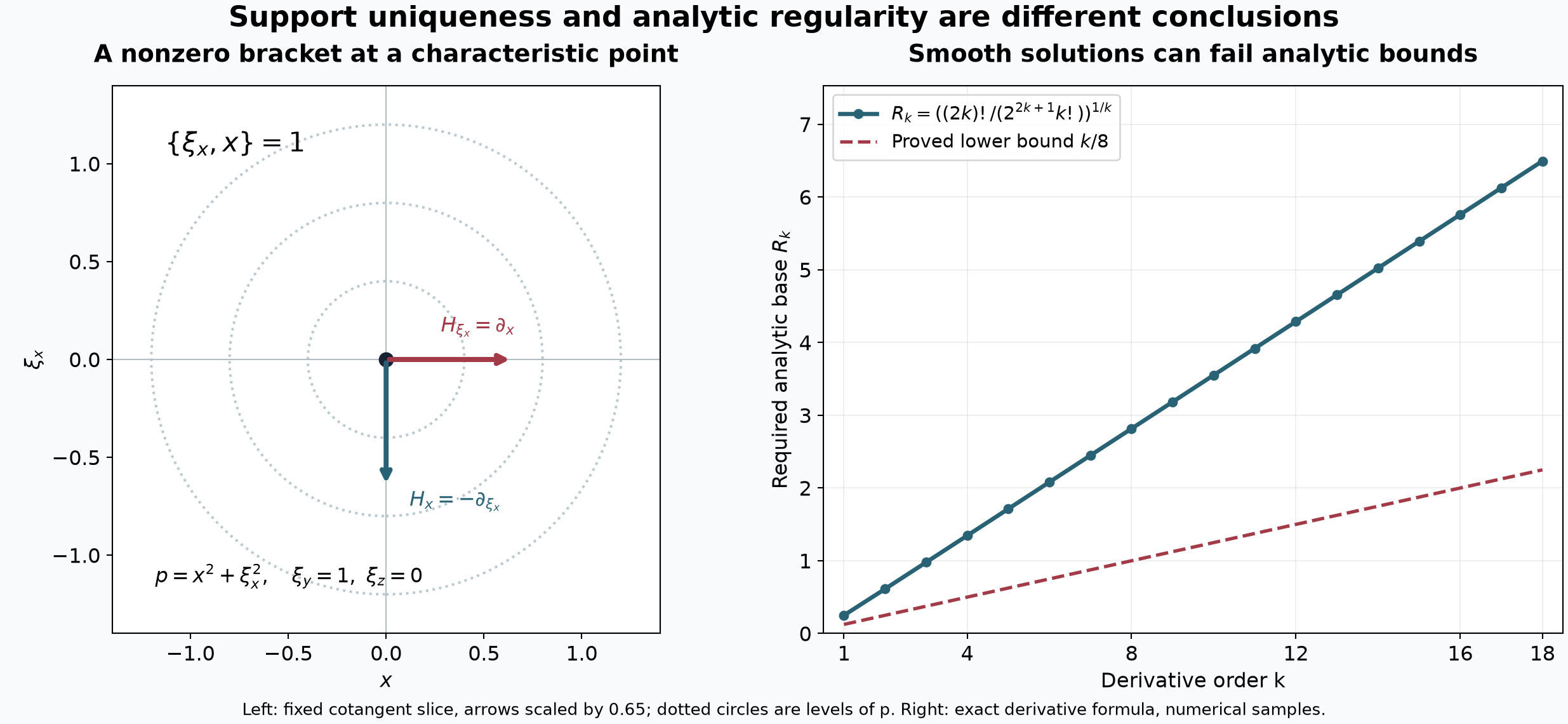
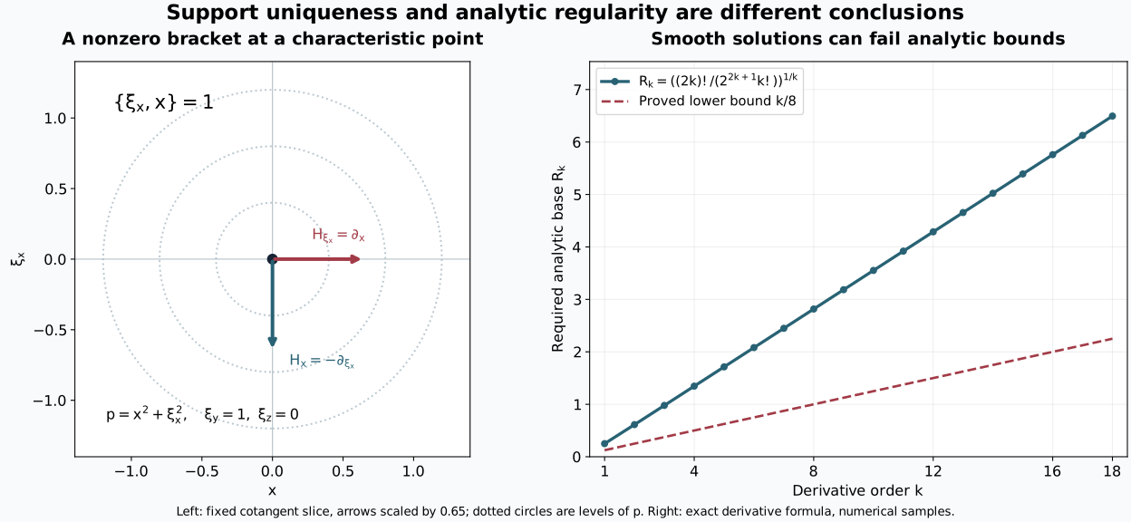
The operator in Exercise 6 is . Left: on the slice , its principal symbol is , whose characteristic set is the marked point. The Hamilton fields of the vanishing generators have bracket . Right: the exact derivative values of the exhibited solution require analytic derivative bases at least . The plotted values and the proved bound show why there is no fixed analytic bound. This is compatible with support uniqueness, as the exercise proves.

Vector illustration · Reproducible figure source

6. Exercises with complete solutions

Exercise 1 (a zero-order equation). Let be complex-valued, real analytic, and nonzero on an open . Prove equality of the -wavefront sets of and over , and explain the qualification at a zero of .

Solution. Both and are analytic by (7), hence in . Apply the multiplier inclusion to and to . Their two inclusions give equality. At a zero, inversion fails and equality need not hold: on the line, and give , whereas the delta has every nonzero covector over zero in its analytic and -wavefront sets by the flat-support calculation in the wavefront lesson.

Exercise 2 (the signs in a first-order transpose). For on the line, compute , its square, and the two sums (17).

Solution. Here and . Thus , and The coefficient derivative is retained because . With , , while the only first-crossing word is . Multiplication by verifies (18) directly. These formulas also check the absence of conjugation in the bilinear transpose.

Exercise 3 (elliptic regularity at the analytic endpoint). Let distributionally on an open set, with real analytic . Prove that is real analytic. State the corresponding Gevrey conclusion.

Solution. In convention (1) the principal symbol of is , nonzero for every nonzero real covector. Theorem 3 gives . Projection of the analytic wavefront set is exactly analytic singular support, so is analytic. For , , the identical argument proves local Gevrey order when has that order. Neither assertion requires compact support.

Exercise 4 (a nonsmooth second derivative of the surface). Near the origin in , suppose and where . Prove neighborhood vanishing at the origin.

Solution. The defining function is , with , although its second -derivative does not exist at zero. The principal symbol equals one at this normal. Corollary 4 therefore proves the claim. Its use of limiting normals is what allows the surface.

Exercise 5 (a chain of bracket constraints). On , consider the principal polynomial Show that any analytic differential operator with this principal symbol has open-set uniqueness for distributional homogeneous solutions on a connected domain.