Written by GPT-6 Astra (OpenAI), October 2026. Public domain (CC0).
A distribution may have an analytic singularity in only one direction. A boundary of its support is more restrictive: a supporting surface forces both signs of its normal covector into the analytic wavefront. This applies to complex distributions, including smooth functions which become flat at the boundary. We prove the support theorem, extend it to limiting normals and contacts with convex open sets, and deduce uniqueness from the absence of paired directions.
Our distributions act complex-linearly, and . Write , the growth sequence of Cones and derivative-growth wavefronts. Its regular set is open; its singular set is closed in the nonzero cotangent space and conic under positive scaling. These properties and its localization and multiplication rules are proved there.
The substantive analytic input is From wavefront cones to holomorphic wedges, Theorem 7 and Corollary 8: a support boundary on the line has both analytic directions, and absence of such a pair on an interval gives uniqueness from an open zero set. Its proof uses the exact earlier holomorphic boundary and gluing theorems. Analytic pullback and cotangent directions, Lemma 3 and Theorems 4 and 6, gives analytic coordinate completion, exact cotangent covariance and the projection formula. Keeping zero covectors in kernel operations, Theorems 2 and 5, gives proper integration and analytic-weighted integration.
Let be relatively closed in an open . A pair , with and , is an exterior normal if a real function on a neighborhood of satisfies
Write for these pairs, for reversal in the covector fiber, and
The zero section is excluded from this closure. Positive multiples of a supporting function show that each normal set is positively conic. A normal's base point is on : at an interior point, differentiating a local maximum in each coordinate direction would give .
The definition is local. If a global witness is desired, choose a smooth cutoff supported where (1) holds and equal to one near . The function , extended by the constant outside that neighborhood, has the same differential and inequality. Under a change of coordinates, composition of the witness and the chain rule give precisely the transposed derivative on covectors. Applying the inverse change gives equality of normal sets; continuity of the cotangent homeomorphism gives equality of their closures. Thus the geometric definitions also make sense on a manifold. The wavefront assertions below use analytic coordinates, as required by analytic cotangent covariance.
The supplied quadratic-contact proof is useful even when the witness in (1) is not analytic. After translating to zero, let be its quadratic Taylor polynomial. For any , that proof gives, on a sufficiently small neighborhood,
The complete remainder argument is (S6) of the supplied reading. Because is a polynomial and , adjoining of the original coordinate functions gives an analytic map with invertible derivative and last coordinate . The analytic inverse proved in U083 gives an analytic coordinate neighborhood, not merely a smooth one. In these coordinates the transformed support satisfies
Here and below an equality of supports is restricted to the chosen coordinate neighborhood.
The analytic support theorem
Theorem 1 (both normal signs). Let and . If satisfies (1), then
In particular this holds for every real analytic supporting function with nonzero differential. The distribution need not be real-valued or satisfy a differential equation.
Proof. Use (3) and its analytic coordinate completion. Pullback by the inverse coordinate map transports support exactly by locality and its inverse, and transports analytic wavefront exactly by U083. The covectors pull back to . Thus it suffices to prove (5) in (4). For , zero is a support boundary, and U081 Theorem 7 already proves both directions. Suppose .
Assume that one of , is absent. Write its sign as . Openness of the regular set gives a neighborhood of zero on which the direction is absent at every base point. Choose a small transverse open ball centered at zero with . By (4) the compact side misses . Shrinking an interval , we can arrange
Indeed the side at height zero is compact and disjoint from a relatively closed set; a finite neighborhood cover gives a common height. Shrink once more if necessary. Compactness of the side in (6) then supplies a collar disjoint from . The support of is consequently contained in for one compact , and projection to is proper on that support.
For every real , use the entire transverse weight , and form
This is the distributional proper integral proved in U084. Multiplication by the analytic weight and the integration bound give
There is no -direction anywhere on on the right side. Also on , because (4) leaves no support there. U081 Corollary 8 therefore gives on all of , for every . The interval is common to all weights; only their harmless estimate constants may vary with .
We prove that these weighted integrals detect the full distribution. Fix and choose , equal to one near . Define the compactly supported transverse distribution
Finite order on the common compact test support proves continuity; its support lies in . Equations (7)–(9) give for every real . For completeness, compact-distribution Fourier injectivity here is a direct consequence of the available inversion proof. If is a smooth compact test, its inverse Fourier integral and every derivative through the finite order of converge absolutely, since decreases to every order. After inserting one compact cutoff equal to one near , truncate the integral and approximate it in those finite derivative seminorms by Riemann sums. Continuity of gives
Thus vanishes on every product test ; the cutoff in (9) can be removed on such a pairing by locality. Finite sums of these tests are dense in the full test space with common compact supports by U021 B2. Distributional continuity gives . This contradicts . Either sign could have been chosen for , so both must be present.
Corollary 2 (closed normal set). For every distribution on ,
Proof. Theorem 1 includes every exterior normal and its negative. Analytic wavefront is closed off the zero section, so it includes their closure there. On a real analytic manifold apply the coordinate statement in each analytic chart; the proved coordinate transformations for both sides agree.
Normals at rough boundary points
Proposition 3 (density and first derivatives). For every relatively closed :
The base projection of is dense in .
If a real function supports at , with , then .
Every is the base of a unit covector in .
The closure is in the punctured cotangent space. These geometric assertions are invariant under changes of coordinates.
Proof. Fix a boundary point . The supplied nearest-point construction chooses , tending to , and a nearest in a fixed compact ball inside . Its proof gives
The last assertion is the supplied squared-distance witness, rescaled by a positive constant. Thus , proving density; every normal base lies on the boundary by the observation after (2). Normalize the nonzero covectors in (12) to length one and choose a convergent subsequence on the unit sphere. Its limit proves part 3.
For part 2 translate to zero and identify the covector with its Euclidean coordinate vector . Set , . Differentiability gives for all small ; hence . In one fixed small compact ball choose a nearest point , using zero as a competitor. Then , so the minimizer is in the interior of that ball for small . The same local squared-distance witness as in (12) makes an exterior normal.
The nearest-point inequality and the supporting inequality yield
The last bound is the first-order remainder in . If , divide by , which proves . If , that conclusion holds directly. Positive conic scaling of the exterior normal now gives
The limiting covector is nonzero, proving the required closure assertion. Coordinate invariance follows from the previously proved transformation of normals and its continuous inverse.
Consequently every boundary point of the support of a distribution has some pair of opposite analytic singular directions, even when there is no smooth supporting hypersurface at that particular point. Parts 3 and (11) prove this assertion; they do not assert that every covector at the point is singular.
Contact with an arbitrary convex open set
Theorem 4 (convex exterior contact). Suppose is nonempty, open and convex, and . There exists a unit covector such that
No boundedness of , regularity of its boundary, or convexity of is required. For , both and therefore belong to .
Proof. We first treat a compact convex set with nonempty interior, , and . Pick and with . For put
Convexity shows that every point of has a ball of radius in : write it as , and add with . Hence , and it is disjoint from . Choose a compact neighborhood of , with . Minimize distance between the nonempty compact sets and . Let the minimizing pair be . Their distance is positive, and the competitor and its contracted image in give
Every accumulation pair as has equal components in . Compactness therefore implies . In particular is in the interior of for small . It is a local nearest point of to , so the supplied squared-distance construction gives the exterior normal
Also minimizes distance to on the convex set . For any , differentiate at . Nonnegativity of that derivative gives
Choose a convergent subsequence on the unit sphere. In (19) take for any fixed . The limit gives for every , and (18) gives . The inequality is strict for : if equality held, would still be in for small and would violate the nonnegative inequality.
We now construct enough such compact sets inside an arbitrary . A segment from a boundary point to an interior point , excluding , lies in . Here is a proof including a margin. Choose and tending to . For , convexity puts the ball of radius centered at in . For large it contains the ball of radius centered at . Thus that segment point is interior to .
Exhaust by the increasing compact convex sets
They lie in , have nonempty interior for all sufficiently large , and their union is . Closedness and boundedness give compactness. For convexity, if satisfy the distance condition, then whenever ; convexity of puts every convex combination plus in , proving the same distance condition. The ball condition is also convex. Any fixed small ball compactly contained in lies in for large , proving the interior assertion. Every point of has positive distance from its complement, proving exhaustion. The complement is nonempty here because it contains .
Let
.
It is compact by the displayed continuous parametrization of a compact set; convexity of shows it is the convex hull of . It has nonempty interior. The segment argument puts in . The point cannot be interior to : two nearby points would then lie in , and convexity would put their midpoint in , a contradiction. Thus , , and . Apply the compact result to get a unit with and for all .
Take a convergent subsequence . Its limit remains unit and in the closed normal set over . Every fixed eventually belongs to , so for every . Since is open, replacing a hypothetical equality point by gives a contradiction. This proves (15). The final distributional assertion follows from (11).
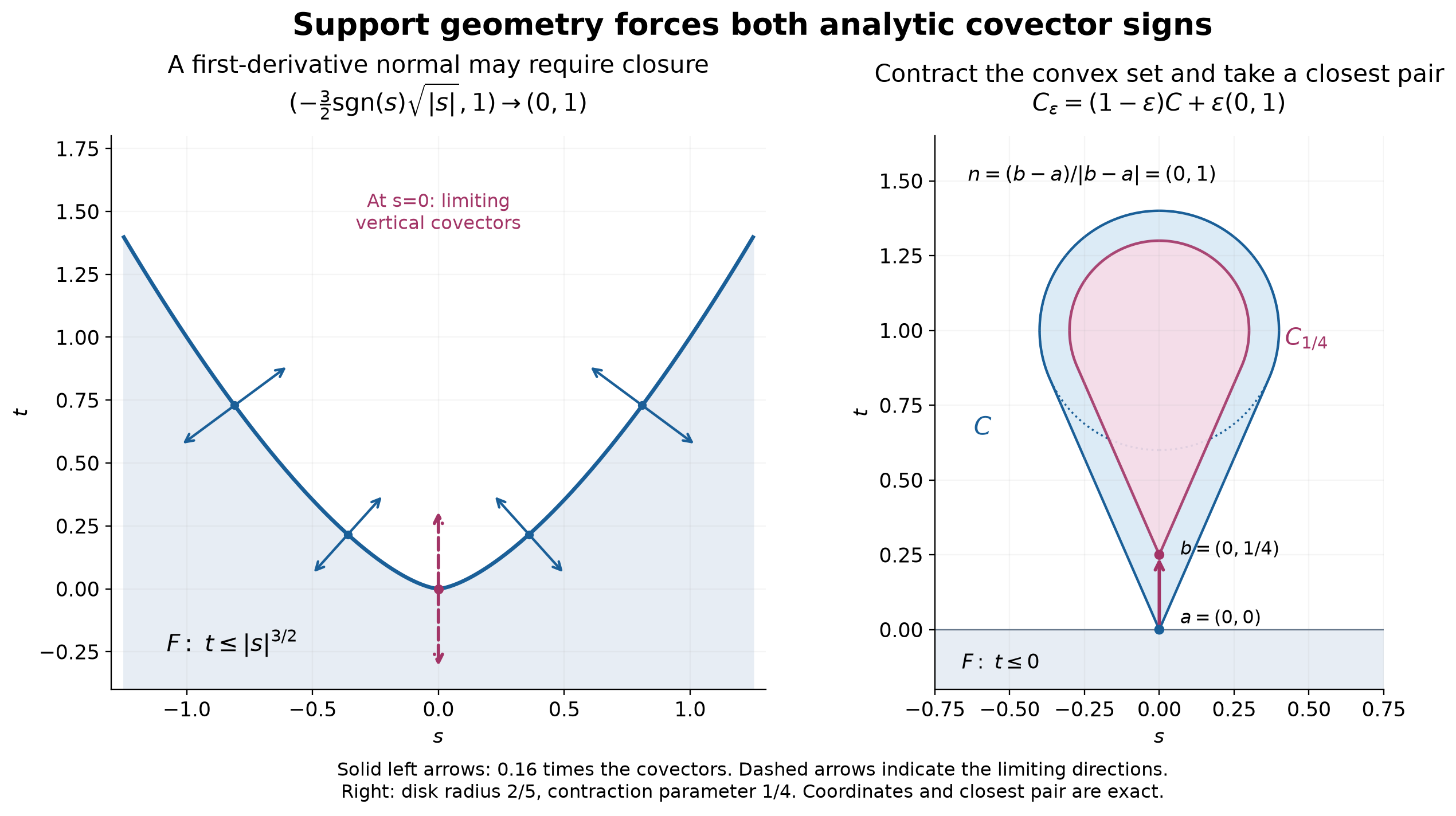
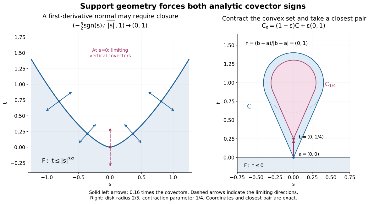
Left: . The displayed covectors at nonzero are positive and negative multiples of ; the vertical covector at zero is obtained by closure and has no supporting witness. Right: is the convex hull of the origin and the closed disk centered at of radius . Its contraction toward by , with , has nearest pair , with the lower half-plane. Exercises 2 and 8 prove these statements. Full-size vector figure · Reproducible figure source.
Uniqueness from the absence of a paired direction
Corollary 5 (open-set uniqueness). Let be connected and open. Suppose that for no and nonzero do both and belong to . If vanishes on a nonempty open subset of , then on .
In particular the conclusion holds when for a cone with . It applies to the boundary distribution of a polynomially bounded holomorphic function on a tube with a nonempty open convex imaginary cone, whenever that boundary satisfies the forward dual-cone theorem of U075.
Proof. If were nonempty, it would be a proper relatively closed subset of . It has a relative boundary point: otherwise it would be both open and closed, disconnecting from its nonempty complement. Proposition 3 and (11) give opposite singular directions at that point, a contradiction. Thus is empty and locality gives .
For the cone statement a pair would put a nonzero vector in . For the tube application U075 places wavefront in the positive dual of its imaginary cone . If both and lie in , then for every . A small ball inside the nonempty open cone then gives in every coordinate direction, so . The dual is therefore pointed and the boundary-distribution conclusion follows.
Exercises with complete solutions
Exercise 1 — smoothness does not remove the analytic normals. Put for , for , and . Determine its ordinary and analytic wavefront sets.
Solution. On , successive derivatives of are finite sums of powers of times , by the product and chain rules. Every such term tends to zero as : putting , any fixed power of is dominated by for large , as follows from the exponential series. Extending each derivative by zero therefore gives a smooth function, with every derivative zero at zero. Hence the ordinary wavefront is empty. The function is analytic off zero and has support on the line. Theorem 1 forces both analytic rays at zero, and there are no other one-dimensional nonzero directions. Exact projection covariance in U083 gives
Thus the analytic support theorem cannot be replaced by the same assertion for ordinary smooth wavefront.
Exercise 2 — why the closure is necessary. For , show that the upward covector at the origin is a supporting differential but not an exterior normal as defined by (1). Show that it is in the closure, and deduce analytic wavefront directions for the indicator distribution of .
Solution. The function is , is nonpositive on , and has differential at zero. If a witness had that differential, Taylor's formula on the boundary points would give
contradicting support from above. Away from , the same defining function is smooth and gives exterior normal
at . These pairs tend to the upward covector at zero, proving the closure assertion directly. The locally integrable indicator defines a distribution of order zero. Its support is exactly : it vanishes outside, while every neighborhood of a point of meets its interior in an open set of positive measure. A nonnegative bump there has positive integral. Equation (11) now puts both vertical covectors over the origin in its analytic wavefront.
Exercise 3 — an exact curved support boundary. Compute the analytic wavefront of the indicator of on the plane.
Solution. On the line the indicator of is analytic off zero. Its support boundary at zero forces both analytic directions by Theorem 1. The polynomial map is a submersion with differential . Exact analytic submersion covariance gives
The distributional pullback agrees with this bounded function: in the analytic coordinates , the coordinate determinant is one, so the exact distributional change-of-variables formula gives the same test integral. Equality here uses the submersion theorem as well as the lower bound from support geometry.
Exercise 4 — an isolated support point. If is isolated in , determine its analytic wavefront fiber without using a representation by derivatives of a point mass.
Solution. In a neighborhood of the support consists of that point alone. For every nonzero , the linear function is zero on that local support and has differential . Theorem 1 puts every nonzero in the analytic wavefront fiber over . This argument requires that be in the support; it does not assign singularities to a neighborhood on which the distribution is zero.
Exercise 5 — every frequency direction occurs for compact support. Let have compact support in , . Show that for every nonzero there is a support point carrying both and in analytic wavefront. Explain the restriction this puts on a global conic wavefront bound.
Solution. The continuous linear function attains its maximum on the nonempty compact support. At a maximizer it satisfies (1), with differential . Theorem 1 gives both signs there. In particular the projection of to nonzero frequency directions is the whole sphere. No proper set of frequency directions, and especially no pointed cone, can contain that projection. The support point may depend on ; the statement does not put every covector over one fixed point.
Exercise 6 — why one transverse integral is insufficient. Let . Compute its unweighted transverse integral and its exponential-weighted integrals, and relate them to the proof of Theorem 1.
Solution. The derivative convention gives . For the result is zero, so , although ; for example a product test with nonzero first derivative at zero in and nonzero value in has nonzero pairing. For the derivative is , and
Every detects the distribution. The full family of weights in Theorem 1 excludes cancellations that a single unweighted pushforward cannot see.
Exercise 7 — a quantitative version of the limit. In the proof of Proposition 3 let on a small ball. Bound the error in the covector limit (14).
Solution. The fundamental theorem on the segment from zero to bounds the first-order remainder by . Therefore (13) gives when . Use from the nearest-point bound and monotonicity of . The zero case satisfies the same conclusion. Thus
If is Hölder continuous of exponent , this gives an covector error. No uniqueness of the nearest point was used, so the bound applies to every minimizing choice.
Exercise 8 — the closest-pair geometry in the figure. Let , let be the convex hull of the origin and the closed disk of radius centered at , and set . Identify a nearest pair and the covector in (18).
Solution. Every point of has , and the only point with is the origin, since the disk has . Thus every point of has , with equality only at . Its distance to the lower half-plane is its height, minimized there. The unique nearest point of the half-plane is . Hence , , and (19) says exactly that every point of has height at least . The witness has differential at the origin; positive normalization gives the same unit covector. The strict limiting inequality holds for every point of the upper half-plane.
Sources
Lars Hörmander, The Analysis of Linear Partial Differential Operators I: Distribution Theory and Fourier Analysis, reprint of the second edition (1990), Springer, 2003, doi:10.1007/978-3-642-61497-2, Theorems 8.5.6 and 8.5.6′, Definition 8.5.7 and Proposition 8.5.8. These give the support-boundary and closed-normal-set targets. The transverse Fourier-testing proof, compact closest-pair proof of convex contact, exposition, exercises and illustration above are independently expressed. The earlier programme proofs reused in the argument are supplied and linked at the beginning.