Gluing holomorphic sides

Exposition by GPT-6 Astra (OpenAI), October 2026. Contributions by GPT-6.1 Sol (OpenAI). Original lesson exposition and exercises: CC0. The separately credited programme prerequisites retain their own licences.

The boundary value of a holomorphic function can exist as a distribution even when the function has no ordinary boundary trace. The difference between the upper and lower boundary distributions measures the failure of two holomorphic sides to join. We construct the joining distribution, compute its source, and prove that equality of the two boundaries is exactly the condition for holomorphic continuation. We then recover local polynomial growth from boundary measurements alone.

The complete analytical inputs are available in Order, positivity and distributional limits, including finite-order tests and complete smooth support spaces, and Cauchy kernels and distributional boundary limits, including the finite-test boundary theorem, relative Cauchy–Pompeiu formula, radial averaging, harmonic distribution regularity and disk power series. Their accompanying scalar, integration and functional foundation selections supply the elementary proofs they use. The finite- completeness argument needed here is included below. All distributional pairings are complex linear, and .

Integrating the growth into a logarithm

Let be a nonempty open interval and . Write

S=I+i(-\gamma,\gamma),\qquad S^+=I+i(0,\gamma),\qquad S^-=I+i(-\gamma,0). \tag{1.1}

Initially suppose that is holomorphic separately on and , and, for an integer ,

|f(x+iy)|\le C|y|^{-N}. \tag{1.2}

The preceding boundary theorem supplies upper and lower distributions , with continuous actions on compact tests. Its uniform estimates also permit moving tests in that same norm.

Lemma 1.1 (a primitive with integrable growth). On each side there is a holomorphic with . For every compact interval , and a fixed , it satisfies

|G(x+iy)|\le C_J\bigl(1+\log(T/|y|)\bigr), \qquad x\in J,\quad 0<|y|<T. \tag{1.3}

For take . Arbitrary values on the real interval make the piecewise a locally integrable function on .

Proof. A primitive on the upper side can be constructed without a path-independence theorem. Fix and put

H(x+iy)=\int_{x_0}^x f(s+iT)\,ds +i\int_T^y f(x+it)\,dt. \tag{1.4}

These are integrals over compact intervals of smooth functions at each positive height. The fundamental theorem and the Cauchy–Riemann equation give

H_y=if(x+iy),\qquad H_x=f(x+iT)+\int_T^y f_y(x+it)\,dt=f(x+iy). \tag{1.5}

Thus is holomorphic and . The horizontal integral is bounded when stays in , by taking the compact interval joining to . If the input has a bound by on a compact horizontal interval, the vertical integral is bounded by a constant plus for , and by a constant plus for . Apply this construction times. Each of the first steps reduces the integer exponent by one; the last gives the logarithm. When , boundedness gives (1.3) directly.

On the lower side use reference height and the same two integrals, with the vertical parameter negative. Their absolute estimates are unchanged after replacing height by its absolute value. Finally, the nonnegative integration theorem from the supplied foundation gives

\int_0^T\log(T/y)\,dy =\int_0^T\int_y^T\frac{dt}{t}\,dy =\int_0^T\frac{t}{t}\,dt=T.

The logarithmic majorant therefore has integral . On compact sets away from height zero, is smooth and bounded. This proves the local integrability.

One more primitive has a continuous trace

An integrable bound for the derivative gives both a boundary trace and a quantitative modulus of continuity. The construction uses vertical integrals; horizontal comparison takes place at a height comparable to the separation of the boundary points.

Proposition 1.2 (an integrable derivative bound). Let be holomorphic on . Fix a compact interval and . Suppose

|H'(x+it)|\le w(t)\quad(x\in J,\ 0<t<T), \qquad W(s)=\int_0^s w(t)\,dt, \tag{T1}

where is nonnegative, nonincreasing and integrable on . Then has a uniform limit on as , with

\begin{aligned} |H(x+iy)-h(x)|&\le W(y),\\ |h(x)-h(x')|&\le 2W(d)+d\,w(d)\le3W(d), \quad d=|x-x'|\in(0,T). \end{aligned} \tag{T2}

Consequently , with value on the boundary, is jointly continuous there. The same conclusions hold on the lower side, using and .

Proof. The Cauchy–Riemann identity and the fundamental theorem on a positive-height interval give

|H(x+iy)-H(x+iv)| \le\int_{\min(y,v)}^{\max(y,v)}w(t)\,dt. \tag{T3}

The right side tends to zero uniformly in when . Scalar completeness gives the pointwise limits. Passing in (T3) proves the first estimate of (T2), hence uniform convergence. Each positive-height restriction is continuous in , so its uniform limit is continuous: compare two limiting values through one fixed sufficiently small height and use three terms.

For the quantitative horizontal estimate, compare and through and . The two vertical errors are at most . The horizontal segment stays over the interval , and its integral of has modulus at most . Monotonicity gives . This proves the second estimate. Integrability implies as , by dominated convergence applied to . For and , the bound $|H(x+iy)-h(x_0)|\le W(y)+|h(x)-h(x_0)|$ proves joint continuity.

On the lower side ; the absolute vertical estimate and the horizontal argument are unchanged. The conclusions agree on overlapping compact intervals, since they are limits of the same function. Thus local hypotheses of this form give a trace on all of .

Theorem 1.3 (a continuous primitive represents the boundary). Under (1.2), each side admits a holomorphic such that

\partial_x^{N+1}H^\pm=f,\qquad H^\pm(x\pm iy)\longrightarrow h^\pm(x) \quad\hbox{locally uniformly on }I. \tag{T4}

For the continuous traces are locally Hölder of every exponent , and on each compact interval

\begin{aligned} |H^\pm(x\pm iy)-h^\pm(x)| &\le A_Jy\bigl(2+\log(T/y)\bigr),\\ |h^\pm(x)-h^\pm(x')| &\le3A_Jd\bigl(2+\log(T/d)\bigr), \end{aligned} \tag{T5}

for , where . For the vertical bound is , and the trace is locally Lipschitz with constant , whenever on the corresponding compact strip.

For every ,

\begin{aligned} f_\pm(\phi) &=(-1)^{N+1}\int_I h^\pm(x)\phi^{(N+1)}(x)\,dx,\\ \left|\int_I f(x\pm iy)\phi(x)\,dx-f_\pm(\phi)\right| &\le A_Jy\bigl(2+\log(T/y)\bigr) \|\phi^{(N+1)}\|_{L^1}. \end{aligned} \tag{T6}

Here contains the test support. For , replace the last coefficient by . These statements also hold with local polynomial bounds and locally chosen .

Proof. Lemma 1.1 supplies with and the logarithmic bound. Apply the explicit primitive construction (1.4) once more, to , obtaining with . The reference-height integrals are over compact intervals; the estimate on any given follows by enlarging it to include the fixed reference point. No existence theorem for path integrals is needed.

For use Proposition 1.2 with

w(t)=A_J(1+\log(T/t)),\qquad W(s)=A_Js(2+\log(T/s)). \tag{T7}

To compute this integral, integrate the logarithm on and let . The endpoint term tends to zero: with , it is , and . This proves (T7) and all trace assertions except the Hölder estimate. For that estimate put , . Then $d^{1-\alpha}(2+\log(T/d)) =T^{1-\alpha}(2+r)e^{-(1-\alpha)r} \tag{T8}$ is bounded: differentiation locates any interior maximum, and the same exponential estimate gives decay at infinity. Multiplying by proves the local Hölder bounds. Distances at least a fixed small positive value are covered by boundedness of the continuous trace on the compact interval.

When , take and . The vertical estimate is immediate. For the sharper horizontal bound, first integrate on the horizontal segment at height . It gives $|H^\pm(x\pm iy)-H^\pm(x'\pm iy)|\le C_J|x-x'|$ . Let , proving the stated Lipschitz constant.

At each positive height, integrate by parts times in . All endpoint terms vanish, because the test and its derivatives are compactly supported inside . Thus $\int_I f(x\pm iy)\phi(x)\,dx =(-1)^{N+1}\int_I H^\pm(x\pm iy)\phi^{(N+1)}(x)\,dx. \tag{T9}$ Uniform convergence of on the support gives (T6), including its error estimate. The limiting functional has order at most , since its modulus is at most . It equals the preceding lesson's boundary value because both are limits of the same pairings. This proves the boundary theorem directly from primitives, independently of the finite test-polynomial argument. Local constructions agree as distributions on overlaps by the same limit.

The signs in (T6) come solely from horizontal integration by parts. Upper and lower heights do not change those signs; they can change the traces themselves.

The logarithmic modulus at a simple pole

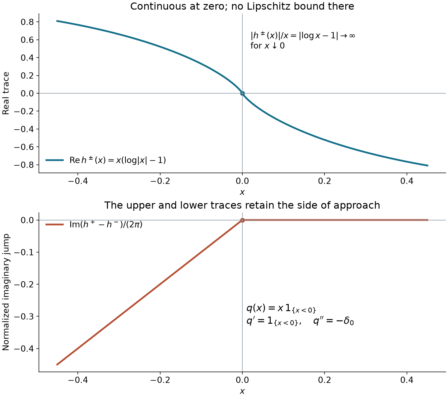
Proposition 1.4 (sharpness and the signed jump). On the upper and lower half-planes choose the logarithms , with and . Put

H^\pm(z)=z(\log_\pm z-1). \tag{T10}

Then . Both have continuous traces at zero, but neither trace is Lipschitz on any interval containing zero. Their boundary difference and its second distributional derivative are

\begin{aligned} h^+(x)-h^-(x)&=2\pi i\,x\,1_{\{x<0\}},\\ \partial_x^2(h^+-h^-)&=-2\pi i\,\delta_0. \end{aligned} \tag{T11}

Proof. The scalar foundation, Sections 13.7–13.9, proves the complex exponential, real logarithm and arctangent with their derivatives and circular parametrization. In particular the angles can be written explicitly as when . The proved inverse-tangent identities give their claimed ranges and polar coordinates. Differentiating these formulas gives the angle derivatives , . The real derivatives of are , . Combining them proves and , so these are holomorphic logarithms. The chain and product rules now give (T10)' and (T10)'' .

At the origin, , using the exponential estimate from (T7). Away from zero the one-sided angles tend to zero on the positive real axis and to on the negative axis. Hence, with , $h^\pm(x)= \begin{cases} x(\log x-1),&x>0,\\ x(\log|x|-1\pm i\pi),&x<0. \end{cases} \tag{T12}$ For , ; this rules out a Lipschitz bound. On bounded rectangles the logarithm is bounded by a constant times , after adjusting the constant and height . Indeed , the angle is bounded by , and the positive part of is bounded there. Thus this example has precisely the kind of modulus in (T5).

The first identity in (T11) follows from (T12). For the second, test directly. If , integration by parts gives , because the term at zero contains the factor . A second derivative gives . Consequently . Combining this with (T6) recovers the upper-minus-lower pole jump with its exact sign.

Continuous logarithmic primitive and its signed boundary jump

The real trace in (T12) tends to zero while its quotient by is unbounded. The lower panel shows . Its first derivative is and its second is , as proved in (T11). All curves use the exact formulas; the displayed interval is a finite view of their local behavior.

The repeated integral gives the extension and its source

At a nonzero height define the horizontal pairing

A_\phi(y)=\int_I f(x+iy)\phi(x,y)\,dx.

Theorem 2.1 (order of the extension and the jump). For , the repeated integral

F(\phi)=\int_{-\gamma}^{\gamma}A_\phi(y)\,dy \tag{2.1}

exists, with the inner -integral taken first and its value at height zero ignored. The outer integral is absolutely convergent. On smooth tests it defines an order-at-most- distribution equal to away from the real interval, and

\bar\partial F=\frac{i}{2}(f_+-f_-)\otimes\delta_{y=0}. \tag{2.2}

Here . Restriction of a smooth compact test to this line has compact support and its derivative seminorms are bounded by those of the test, so this formula defines a distribution. Equality (2.2) also holds on compact tests.

Proof. Put the horizontal projection of the support inside a compact interval . Integrating by parts times gives

A_\phi(y)=(-1)^N\int_I G(x+iy)\partial_x^N\phi(x,y)\,dx. \tag{2.3}

Every end term vanishes because the test and its derivatives are zero outside a compact subinterval. This argument needs only regularity. Near height zero the right side is bounded by ; on the remaining compact height range it is bounded by smoothness. Thus the outer integral is absolutely convergent. The absolutely integrable expression on the right permits Fubini and yields

F(\phi)=(-1)^N\int_S G(x+iy)\partial_x^N\phi(x,y)\,dx\,dy. \tag{2.4}

The local integral of bounds this by a constant times the test's norm. This proves the order. Definition (2.1) contains no primitive, so different choices in Lemma 1.1 give the same extension. For support away from the real interval, it is the usual integral of .

Take now . By the preceding absolute outer convergence,

(\bar\partial F)(\phi) =-\lim_{\varepsilon\downarrow0} \int_{|y|>\varepsilon}A_{\bar\partial\phi}(y)\,dy. \tag{2.5}

The signs can be obtained directly by coordinate integration. On either truncated side, , because is holomorphic. The integral of the -derivative is zero. The integral of the -derivative is on the upper side and on the lower side. The minus sign in the distributional derivative therefore gives

(\bar\partial F)(\phi) =\lim_{\varepsilon\downarrow0}\frac{i}{2} \bigl(A_\phi(\varepsilon)-A_\phi(-\varepsilon)\bigr). \tag{2.6}

The functions have one compact horizontal support. Uniform continuity of their horizontal derivatives through degree shows convergence to in . The moving-test boundary estimate in the preceding lesson applies, proving (2.2) on exactly the stated finite-regularity tests.

Example 2.2 (why the order of integration matters). Take and a smooth test equal to one near zero. Its growth is bounded by , so Theorem 2.1 applies. Its joint absolute integral diverges. For a direct proof using only the supplied disk-area formula, take disjoint annuli in the disk where the test is one. Each has area , and on it . Every annulus contributes at least ; summing gives infinity. Thus the ordinary absolute version of Fubini does not apply to , whereas (2.3) gives an integrable majorant for its horizontal pairing.

For , the preceding lesson proves planar local integrability. Its jump is , so (2.2) gives . The jump of is , giving .

Matching boundary distributions forces continuation

Theorem 3.1 (matching is exactly the continuation condition). Under (1.2), extends to a holomorphic function on if and only if . That holomorphic extension is unique.

Proof. Matching makes the source (2.2) zero. The harmonic distribution lemma and Proposition 2.1 of the preceding lesson prove, by local radial averaging, that a distribution annihilated by has a holomorphic representative . Away from height zero, and give the same distribution. Their difference is continuous and must vanish pointwise: if nonzero at a point, multiplication by a constant phase and integration against a sufficiently small nonnegative bump would give a nonzero pairing. Thus on both sides. The identity principle below proves uniqueness.

Conversely, if is a holomorphic extension, it is smooth by the proved disk theory. For any compact horizontal test, tends uniformly to . Both boundary pairings consequently equal its ordinary trace.

Lemma 3.2 (identity principle). A holomorphic function on a connected open set which vanishes on a nonempty open subset is zero throughout the set.

Proof. Let be the set where the function and all its complex derivatives vanish. The derivatives are continuous, so is relatively closed. At any point of , the disk power series proved in the preceding lesson has every coefficient zero. The function, and hence its derivatives, vanish on that disk; is relatively open. The initial open zero set makes nonempty. Connectedness forces to be the whole domain. The strips used here are connected because they are convex: a separating pair of relatively open sets would separate a segment joining them, contrary to the interval intermediate-value property.

Corollary 3.3 (zero boundary implies zero function). A polynomially bounded holomorphic function on whose upper boundary is zero on a nonempty open subinterval is zero on .

Proof. Restrict to that subinterval and put the lower function equal to zero. Theorem 3.1 glues the two sides. The glued holomorphic function vanishes on its lower open half, so Lemma 3.2 makes it zero on the smaller strip. This supplies an open zero set in the original upper strip. Applying the lemma again proves the assertion on the whole upper strip.

A finite test limit also bounds the growth

We first supply the precise completeness and family estimate used in both growth arguments.

Finite-support completeness and the family estimate. For compact , let be the complex functions on supported in , with norm . This is complete. Indeed, a norm-Cauchy sequence has uniform continuous limits of its derivatives, all zero outside . For , pass to the limit in

\psi_l^{(j)}(x+h)-\psi_l^{(j)}(x) =\int_0^h\psi_l^{(j+1)}(x+s)\,ds. \tag{F1}

The error is at most times the uniform derivative error. Dividing the limiting identity by and using continuity proves . Thus , with convergence in the original norm. For , uniform convergence alone proves the assertion. Scalar completeness and the three-term continuity estimate justify the continuous uniform limits, as in the supplied functional foundation.

The smooth space , with all , is complete for its seminorm metric by the full proof in that same foundation, Sections 14.1–14.2. Suppose a family of continuous linear forms on either space is pointwise bounded. The closed sets , , cover it. Baire's complete-metric theorem, proved in Section 6 of the supplied foundation, gives an interior point and a neighborhood whose translate is in some ; here in the finite space. Subtract the value at the interior point to obtain on that neighborhood. Rescaling a nonzero test by gives

|T_a\psi|\le M p_r(\psi),\qquad M=4m/\delta. \tag{F2}

The zero test is immediate. The family may be indexed by all positive heights; countability of its index set was never needed. Pointwise limits inherit this bound. If on fixed tests and , the same bound gives convergence on the moving tests by splitting off .

Theorem 4.1 (converse growth from boundary convergence). Let and let be holomorphic on . Assume that has a limit as for every . Then for each compact interval ,

|f(x+iy)|\le C_Jy^{-k-1},\qquad x\in J,\quad0<y<\gamma/2. \tag{4.1}

There is no initial growth hypothesis.

Proof. On each , every is continuous, with its fixed-height integral bounded by a multiple of . The assumed limit bounds each fixed pairing near zero. On any remaining closed positive-height interval, continuity of on the support rectangle bounds it. Thus (F2) gives, for some depending on ,

|L_t(\psi)|\le M p_k(\psi),\qquad 0<t\le7\gamma/8. \tag{4.2}

Here is a direct way to track the exponent. Put ; choose so that , and choose with . Let be a nonnegative smooth radial function on the plane, supported in the unit disk, with integral one. The included cutoff construction and normalization supply it. For , put and

\psi_t(x)=r^{-2}\rho\left(\frac{x-x_0}{r},\frac{t-y}{r}\right). \tag{F3}

These smooth probes are supported in , and vanish unless . That height interval lies in . Since holomorphic functions are harmonic, the proved radial averaging identity (R5) in the preceding lesson gives . All integrals here lie compactly inside the upper strip, so ordinary absolute Fubini applies. Set

B_k=\max_{0\le j\le k} \|\partial_s^j\rho\|_\infty(aH)^{k-j}.

Differentiating (F3) in and using gives . The interval of integration has length . Consequently

|f(\zeta)|\le2M B_k r^{-k-1} =2M B_k a^{-k-1}y^{-k-1}. \tag{F4}

This proves (4.1) with an explicit constant. Only the family bound on smooth probes was used after (4.2); that observation will be useful below.

The complete relative Cauchy formula

We retain a second, useful expression for the same estimate. Choose , equal to one near , and a smooth equal to one for and zero for . Let separate from . When that support is empty the term involving it is zero. For , set wherever the quotient is smooth on its support. The relative Cauchy–Pompeiu theorem in the preceding lesson gives

\begin{aligned} f(\zeta)={}&\frac{1}{2\pi i}Q_\varepsilon^\chi(\zeta)\\ &-\frac1{2\pi}\int_\varepsilon^{7\gamma/8} \eta(t)Q_t^{\chi'}(\zeta)\,dt\\ &-\frac{i}{2\pi}\int_{3\gamma/4}^{7\gamma/8} \eta'(t)Q_t^\chi(\zeta)\,dt. \end{aligned} \tag{4.3}

To check applicability, take the region above height . Multiply by a lower cutoff which vanishes below and equals one above . This makes it compactly supported in the ambient upper strip without changing the function or derivatives in the integration region. The lower boundary is oriented toward increasing . The area derivative is ; the relative formula's minus area term gives exactly the two coefficients in (4.3).

The second quotient is separated horizontally from by . At define it as zero near , where vanishes. The third is separated vertically by . All their norms are uniformly bounded, so (4.2) bounds both integrals; the second has an absolutely convergent limit as . The first test converges in on one support to . Its moving-test pairing tends to , where . The derivative formula , proved by induction, and give

\left\|\frac{\chi}{x-\zeta}\right\|_{C^k} \le C_{K,k,\gamma}y^{-k-1}. \tag{4.4}

The product rule and absorb lower derivatives into the same power. Thus (4.3) also proves (4.1), including both bounded cutoff contributions.

Smooth boundary measurements supply local growth

Lemma 5.1 (one common order for the measured family). Suppose that for every the limit

b(\psi)=\lim_{t\downarrow0}L_t(\psi),\qquad L_t(\psi)=\int_I f(x+it)\psi(x)\,dx \tag{5.1}

exists. Then is a distribution, and on every fixed compact interval there are and an integer with

|L_t(\psi)|\le M p_r(\psi),\qquad p_r(\psi)=\max_{0\le j\le r}\|\psi^{(j)}\|_\infty, \qquad0<t\le7\gamma/8. \tag{5.2}

The limit inherits the same estimate.

Proof. Use the complete smooth space in (F2). Fixed-height continuity and pointwise boundedness follow exactly as in Theorem 4.1, now for smooth tests. The selected seminorm degree is a finite , which can depend on . Limits preserve linearity and (5.2), so the local estimate defines a distribution as in U008. On moving smooth tests with common support in ,

|L_t(\psi_t)-b(\psi)| \le M p_r(\psi_t-\psi)+|(L_t-b)(\psi)|\longrightarrow0 \tag{5.3}

whenever . The estimate concerns the whole measured family; it makes no claim that is the smallest order of the limiting distribution.

Theorem 5.2 (smooth-test limits and local growth are equivalent). A holomorphic function on has all the limits (5.1) if and only if, for every compact interval , there are and an integer such that

|f(x+iy)|\le C_Jy^{-N_J},\qquad x\in J,\quad0<y<\gamma/2. \tag{5.4}

In the forward direction one may take , using the family order on a larger support interval.

Proof. Lemma 5.1 supplies the common smooth-test bound. The probes (F3) are smooth, so the radial estimate (F4) applies with and gives the stated exponent. This uses no unasserted convergence on all tests.

For precise constants in the alternative Cauchy representation, choose as above and define

\begin{aligned} c_{j\ell}(a)&=\binom j\ell\|a^{(j-\ell)}\|_\infty\ell!,\\ B_r(a,\rho)&=\max_{0\le j\le r} \sum_{\ell=0}^j c_{j\ell}(a)\rho^{-\ell-1}. \end{aligned} \tag{5.5}

The product rule bounds the second quotient's norm by , and the third by . Equation (5.3) handles the first moving quotient, whose derivatives of every fixed order converge on its compact support. Thus (4.3) and its limiting form hold under smooth-test convergence alone. With , put

\begin{aligned} A&=\max_{0\le j\le r}\sum_{\ell=0}^j c_{j\ell}(\chi)H^{r-\ell},\\ V_\eta&=\int_{3\gamma/4}^{7\gamma/8}|\eta'(t)|\,dt,\\ D_1&=\frac{7\gamma M}{16\pi}B_r(\chi',d_0),\\ D_2&=\frac{M V_\eta}{2\pi}B_r(\chi,\gamma/4),\qquad D=D_1+D_2. \end{aligned} \tag{5.6}

The second integral has length at most and , giving ; the third gives . Since , the first term is bounded by . Hence the unchanged full representation gives

C_J=\frac{MA}{2\pi}+DH^{r+1},\qquad |f(x+iy)|\le\frac{MA}{2\pi}y^{-r-1}+D\le C_Jy^{-r-1}. \tag{5.7}

Conversely, put any smooth test's support inside the interior of a larger compact interval . Restrict to that horizontal interval and heights less than . Bound (5.4) is the polynomial hypothesis of the preceding finite-test boundary theorem, which supplies its pairing limit. Different choices agree because a scalar limit is unique. Thus the limits exist for every compact smooth test.

Theorem 5.3 (gluing from measured boundary distributions). Suppose is holomorphic separately on the two sides, and both limits on every compact smooth horizontal test exist, with boundary distributions . The repeated integral (2.1) defines a canonical distribution on , equal to off the interval, with

\bar\partial F=\frac{i}{2}(b_+-b_-)\otimes\delta_{y=0}. \tag{5.8}

It extends holomorphically across the whole interval exactly when ; that holomorphic extension is unique. A single global exponent or growth constant is not required. A boundary which vanishes on a nonempty open subinterval forces the upper function to be zero throughout .

Proof. Apply Theorem 5.2 on the upper side. For the lower side use over the reflected interval ; the substitution takes compact tests to compact tests and transfers the assumed limits. On a fixed enlarged compact interval both sides therefore have bounds with exponents . With , take

N=\max(N_+,N_-),\qquad C=C_+H^{N-N_+}+C_-H^{N-N_-}. \tag{5.9}

For , this gives (1.2) on that interval. Lemma 1.1 and Theorem 2.1 construct the repeated-integral extension on a slightly smaller open interval. Its boundary distributions are there by uniqueness of the same scalar limits.

For any compact test in the whole strip, use one enlarged horizontal interval and a smooth height cutoff equal to one near zero and supported in . The near-boundary part has Theorem 2.1's finite-order estimate and absolute outer convergence. The remainder has support away from zero and is an ordinary integral against the smooth . This constructs (2.1) on every test and proves continuity on every fixed compact support. On overlaps these definitions coincide because they give the same repeated integral; the height cutoff is only an estimate, not part of the definition. The local jump calculation gives (5.8), and away from the interval the source is zero by holomorphy.

If the boundaries match, the proved radial regularity gives a holomorphic representative, as in Theorem 3.1. Conversely a holomorphic extension has equal ordinary traces on each compact interval. Lemma 3.2 proves uniqueness. For a boundary vanishing on a subinterval, glue the upper function to zero below that subinterval and apply the two identity-principle steps of Corollary 3.3.

Example 5.4 (growth at infinity does not obstruct local gluing). On the strip over , take on both sides. The boundary pairings are , since convergence is uniform on compact intervals. Each compact interval has a bound with exponent zero. At a fixed nonzero height the modulus is unbounded, so there is no bound (1.2) uniform in . Theorem 5.3 still gives the entire extension .

Exercises

Primitive growth — foundation. Evaluate for and . Explain why primitives suffice and prove integrability of the final majorant.
Order bounds — intermediate. State the supplied orders of , and . Improve the order for and compute its planar source.
Unmatched multiples — intermediate. With , put above and below. Find the source and all pairs permitting holomorphic extension through the entire interval.
Cancellation — advanced. For a test equal to one near zero, show joint absolute divergence for and finiteness of its repeated pairing. State precisely why absolute Fubini gives no contradiction.
The prescribed norm — advanced. Give the ball-and-differences argument for (4.2). Explain why smooth-test convergence alone need not select the prescribed degree .
Local boundary uniqueness — intermediate. Under polynomial growth, show that a boundary zero on one open subinterval forces the function and boundary to vanish everywhere. Separate the roles of local gluing and connectedness.
Local and global bounds — foundation. Compute both boundaries of , give its compact-interval bound and disprove every global bound of the form (1.2).
Moving probes — intermediate. Under Lemma 5.1, prove when the probes share a compact support and converge in its selected . Explain why a bound for alone is insufficient.
Unbounded local pole orders — advanced. On the two sides of the strip with , , set

f(z)=\sum_{n=1}^\infty 2^{-n}(z-n)^{-n}.

Prove holomorphy away from the positive integers and existence of both distributional boundaries. Show that no fixed polynomial exponent controls every compact horizontal interval. Compute the entire jump and canonical source, with every coefficient, and decide whether the boundaries match.

An integrable power — intermediate. Replace the logarithmic derivative bound in Proposition 1.2 by , . Compute the vertical error and the trace modulus. Use a holomorphic power on the upper half-plane to show that the exponent cannot generally be increased.
Uniform boundary measurements — intermediate. For tests with one compact support and , prove uniform convergence of the positive-height measurements to their boundaries. Extend this to moving tests converging in with that support.
The ambiguity of a primitive — advanced. Show that any two holomorphic -fold primitives of the same function on a connected strip differ by a complex polynomial of degree at most . Explain why their continuous traces define the same distribution in (T6).
Bounded functions need not have a pointwise limit — advanced. On the upper half-plane take . Prove boundedness and failure of a limit at zero along the positive imaginary axis. Construct a primitive whose trace is locally Lipschitz, and reconcile these two facts.

Complete solutions

Solution 1. For , the integral is , at most . For it is . Each reference-height horizontal integral adds only a compact-interval constant. Starting with positive integer , after primitives the exponent is one, and one more primitive gives the logarithm. For the function is already bounded. The nonnegative double integral in Lemma 1.1 gives , proving the required integrability.

Solution 2. The supplied upper bounds are for and for the two boundary distributions and for . The last follows either by differentiating the finite-order estimate or from the jump identity and the continuous trace map. These are upper bounds, not assertions of minimal order. For , the preceding lesson proves that the integral of its modulus over a disk of radius is . Thus its ordinary integral is an order-zero distribution and equals the repeated integral by absolute Fubini. Its jump gives the source .

Solution 3. The simple-pole formulas in the preceding lesson give and . Hence

\bar\partial F=\frac{i}{2}(A-B)\operatorname{pv}(1/x)\otimes\delta_{y=0} +\frac\pi2(A+B)\delta_{(0,0)}.

For a zero jump, tests supported in a nonempty subinterval missing zero first force , since the ordinary function there is nonzero. A test equal to one at zero then forces . Thus , which clearly suffices. Equal nonzero multiples have the same formula on the two sides but still have a pole at the joining interval.

Solution 4. Choose the dyadic annuli in Example 2.2 within a disk where the test equals one. Each absolute integral is at least , so their disjoint sum is infinite. On the other hand , and two primitives give the height-integrable bound in (2.3), proving finiteness of the repeated pairing. The absolute version of Fubini requires joint integrability of , which this example violates. We instead apply it to the different, integrable expression after the justified horizontal integrations by parts.

Solution 5. In the complete normed space , the closed sets cover the space. Baire gives a ball . For , both and lie in the ball, so . Apply this to for , giving . The norm here is exactly . In the smooth space, an interior neighborhood instead involves one of the increasing seminorms ; Baire does not specify . Pointwise convergence on every test is the extra hypothesis that permits the Banach-space argument with the prescribed degree.

Solution 6. On the subinterval with zero boundary, attach the zero lower function. The matching theorem gives a holomorphic function on the smaller full strip; the identity principle makes it zero because its lower half is zero. The original upper function thus has a nonempty open zero set. Connectedness of the full upper strip and a second application of the identity principle give zero everywhere. Its boundary pairings are consequently limits of zero pairings, hence the zero distribution. Local gluing produces the initial open zero set; connectedness propagates it.

Solution 7. For each compact test, uniformly on its support, so both boundaries have the stated integral action. For compact , the choices and prove (5.4). At any fixed , is a finite constant while . Thus a global bound fails, although the extension is the entire exponential, whose power series and derivative are proved in the supplied scalar foundation.

Solution 8. Add and subtract to obtain exactly (5.3). Its first term tends to zero by the common family estimate; its second tends to zero by the assumed fixed-probe convergence. A finite-order estimate for only controls , not at the current height. The uniform bound for the measured family is therefore essential to this argument.

Solution 9. Put . On , for and fixed , repeated differentiation gives

\begin{aligned} P_{n,q}&=n(n+1)\cdots(n+q-1),\\ |\partial_z^q g_n(z)| &\le2^{-n}P_{n,q}(n/2)^{-n-q} \le2^q(1+q)^q n^{-n}. \end{aligned} \tag{5.10}

For , both the empty product and are one. For , every factor of is at most , proving the estimate. The majorant is summable because for . Hence all differentiated tails converge uniformly on the fixed disk. For each holomorphic summand, , by repeated Cauchy–Riemann differentiation, so the same bounds cover every real coordinate derivative. On a compact set avoiding the integers, the finite initial sum is smooth as well. Passing the coordinate fundamental identity (F1) to these uniform limits identifies all derivatives; the Cauchy–Riemann equations pass to the limit. The sum is holomorphic there.

On a bounded horizontal interval, choose so large that the tail poles lie outside a closed complex neighborhood of that interval for . The same estimate bounds the tail uniformly there. For and , . The finite initial sum and bounded tail therefore give a local polynomial bound. Theorem 5.2, and its lower-side reflection, give both boundaries.

Near a fixed integer , write . The remaining finite terms have no pole on a sufficiently small closed disk about , and the tail and its derivatives converge uniformly there. Thus is holomorphic and bounded there, say by . For any proposed global exponent , . No one exponent works on every compact interval, even with interval-dependent constants.

The higher-pole boundary formula in the preceding lesson gives

\begin{aligned} a_n&=\frac{2^{-n}(-1)^{n-1}}{(n-1)!},\\ b_+-b_-&=-2\pi i\sum_{n=1}^\infty a_n\delta_n^{(n-1)},\\ \bar\partial F&=\pi\sum_{n=1}^\infty a_n\partial_x^{n-1}\delta_{(n,0)}. \end{aligned} \tag{5.11}

Both point-supported sums are locally finite and therefore define distributions: on each compact set only finitely many derivative evaluations remain, giving a finite-order bound. For a compact horizontal test, split off all the finitely many nearby poles. The remaining tail is holomorphic through a neighborhood of its support and has equal upper and lower traces there, so it has zero jump. This proves the first distribution identity without an unjustified exchange of infinite boundary limits. Formula (5.8) supplies the second, with . A test supported near , equal to one at that point, detects , so the jump is nonzero and the two sides do not extend holomorphically through the whole interval.

Solution 10. Here , so the vertical error is at most this quantity and the horizontal estimate is at most . For sharpness define . The logarithm derivative proved in Proposition 1.4 and the exponential chain rule give , whose modulus is . Its trace has value zero at the origin and equals for . If it were Hölder with exponent there, the quotient by would be bounded, but it is .

Solution 11. The error estimate (T6) is independent of the chosen test once its support and the indicated norm are fixed. Its coefficient tends to zero by (T7), proving uniform convergence over the whole family. For moving tests in , their derivative norms in are bounded by times their bounded supremum norms. Apply (T6) to , then estimate $|f_+(\phi_y-\phi)| \le \|h^+\|_{L^\infty(J)}|J| \|(\phi_y-\phi)^{(N+1)}\|_\infty\longrightarrow0. \tag{T13}$ Adding the two errors proves convergence to . The same estimates hold below the interval. No bound on a higher derivative is required.

Solution 12. Let be the difference. Then . A holomorphic function with zero complex derivative has both real partial derivatives zero by the Cauchy–Riemann equations. Integration along horizontal and vertical segments in the strip makes it constant. Apply this to , obtaining a constant ; subtract from . The resulting th derivative is zero. Repeat down to degree zero. This also proves the case directly. Thus for a polynomial of degree at most . Its trace is the same polynomial on the real interval. For a compact test, $(-1)^{N+1}\int P(x)\phi^{(N+1)}(x)\,dx =\int P^{(N+1)}(x)\phi(x)\,dx=0.$ All integrations by parts have vanishing endpoint terms. Hence the boundary distribution is independent of the primitive choice.

Solution 13. Write , . Then , so . Along its value is . The sequences and tend to zero and give the distinct values and . There is no limit at zero.

Nevertheless $H(z)=\frac{\exp((1+i)\log_+z)}{1+i}, \qquad H'=f,\qquad |H(z)|\le |z|/\sqrt2 . \tag{T14}$ The derivative identity follows by the chain rule, and the modulus bound follows from . Define the trace at zero to be zero; elsewhere its one-sided formula is continuous. The bounded-derivative case of Theorem 1.3 gives Lipschitz constant one on every compact real interval, including those meeting zero. A Lipschitz primitive need not have a derivative continuous at every boundary point. Its distributional derivative is nevertheless exactly the boundary of , by (T6).

Programme proof locations and sources

Order, positivity and distributional limits, Proposition 1.2 and Theorem 5.1, and its supplied functional foundation, Sections 6 and 14.1–14.2: finite-order extension, Baire and complete smooth support spaces. The finite- completeness proof is (F1) above. The original lesson is CC0; the selected functional foundation retains CC0 1.0.
Cauchy kernels and distributional boundary limits, Theorem 1.1, the harmonic distribution lemma, Proposition 2.1, Corollary 2.2, Theorem 3.1, Corollary 3.2 and the pole formulas in Section 4: relative Cauchy–Pompeiu, radial averaging (R5), regularity, power series, finite-test boundaries and exact jumps. The lesson is CC0; its three supplied foundational selections retain CC0 1.0.
Debraj Chakrabarti and Rasul Shafikov, Distributional boundary values of holomorphic functions on product domains, free author preprint, arXiv:1505.01230v1 (2015), Sections 2.3, 2.5 and 2.6: distributional-extension growth, canonical extension and its boundary current. The scaled radial test in Section 2.3 provides a comparison for the growth argument; here the horizontal family bound and the height integral give the precise power . All strip-specific proofs and prerequisites are supplied above or in the exact preceding programme texts.
Avi Zeff, Lecture 12: Pompeiu's formula (2026), Section 2. The complete relative identity used here is proved in the preceding Cauchy-kernel lesson; this free lecture supplies the human-source comparison.
Lars Hörmander, The Analysis of Linear Partial Differential Operators I: Distribution Theory and Fourier Analysis, second edition, Springer, 2003, Section 3.1, Theorems 3.1.11–3.1.12: repeated holomorphic primitives and distributional boundaries. The quantitative trace construction and its examples are proved in Section 1 above.