Exposition by GPT-6 Astra (OpenAI), October 2026. Contributions: GPT-6.1 Sol (OpenAI). Original exposition: CC0. Supplied foundations retain their stated licences.
The forward cone bounds every summand contributing to a compact output region. This makes convolution an algebra in which a normalized wave kernel is an inverse. Higher wave powers, complex constant potentials and complex drifts can then be treated on the whole space, including the point source at the vertex.
The full entire Riesz construction used here is U027, Lemma 4.0 and formulas (4.0a)–(4.0h). Its proof includes boundary and vertex integrability, compatible continuation, the exact origin delta, Gamma duplication and linear distribution substitution. Its one-dimensional input is U022, §1, formulas (1.3)–(1.6), and Theorems 2.1–2.2. The Gamma foundations, (G0)–(G2) and (W4a)–(W4e), supply the reciprocal Gamma function and its zeros and recurrence; the angular foundations, A4–A5, supply polar integration and the Gaussian constant.
Proper convolution, derivative transfer, associativity and continuity are fully proved in U021, B0–B3, Theorems 1.1, 3.1–3.2 and Corollary 3.4. Finite-order continuity is U008, Proposition 1.2. For scalar operations we use the calculus foundations, §§12, 13.1–13.5 and 13.7–13.10, and the integration foundations, §§15.0–15.2 and 16. The local holomorphic series and identity principle are U013, Corollary 2.2, and U014, Lemma 3.2. Pairings are complex linear. No growth condition at infinity is imposed.
The normalization of every wave power
Let , with coordinates , and set
Write for the spacetime family of U027 Lemma 4.0; this notation is distinct from the one-dimensional family in U022. The proved global identities are
For , its density is
In U027, absolute spatial integration reduces the vertex condition to integrability of . Continuation is , with overlapping definitions proved equal. Coordinate multiplication forces to be a point mass, and its explicitly evaluated time marginal gives mass one. Thus (1.1) includes the vertex.
We first explain the cone expression away from that vertex. Define
initially for , continued by U022 formulas (1.3)–(1.6) and their proofs. In its notation this is the scalar family at parameter ; in particular
for integers .
On , coordinates have the explicit inverse
Here is the substitution justification. For a continuous on a compact interval, put . The FTC and chain rule give ; integrating proves substitution for a smooth increasing . Apply this for fixed with , on intervals in , then use Fubini. For a singular but integrable power at , apply the same calculation off a deleted neighborhood and pass to the limit in the absolute integrals. The exponents make that passage integrable.
The positive square root is continuous by its monotonicity and the identity
The denominator stays bounded below near . Dividing by gives ; induction through this formula proves smoothness on the positive half-line.
For , extend
by zero wherever the square root is unavailable. This extension is smooth and compactly supported: the original support has , so the expression is identically zero near ; its coordinate image is compact. Differentiation under its compact -integral is the parameter-integral proof in U021 B1. Define the distribution on by
The transformed test has common compact support and bounded seminorms when does, so this is a distribution and is entire in . In the integrable range it agrees with the ordinary composed density. Comparison with (1.2) and the scalar identity principle therefore give, on ,
for every parameter, with understood as its entire reciprocal. No critical substitution at the vertex is required.
Theorem 1.1 (forward inverses of the wave powers). For every integer , the unique -supported fundamental solution of is
On it has the cone expression
At the vertex, the notation means the global distribution (1.3). If is odd and , its exact support is the closed boundary . In every other case its exact support is . For every cone-supported distribution , is the unique cone-supported solution of .
Proof: normalization and support. Iterating (1.1) gives . The preceding coordinate construction and give (1.4), with its exact coefficient.
For odd and , the scalar factor is
.
It is zero off . It is nonzero in every neighborhood of a nonvertex cone point: choose small coordinate product supports about , and a test of the form
within that chart, where and . Its transformed integrated test is , so its pairing is a nonzero multiple of that derivative. Such supports can be arbitrarily small, because and . A cutoff supported in and equal to one on the positive inverse image makes the displayed expression a global test there. This proves that all nonvertex cone points belong to the support. There is no interior support, by the same scalar formula; off-cone support is excluded by (1.1). Closedness adds the vertex and gives exactly .
For the remaining odd-dimensional cases the scalar exponent in (1.4) is a nonnegative integer, so the interior density is nonzero. For even it is a half-integer. The reciprocal Gamma normalization is nonzero at that half-integer plus one, since its only zeros are the nonpositive integers, as proved in the supplied Gamma foundation. Thus the interior density is again a nonzero smooth power. A nonzero continuous density has nonzero pairing on a sufficiently small nonnegative bump after multiplication by a constant phase; hence every interior point belongs to the support. Closedness and (1.1) give .
Proof: all sources and uniqueness. Addition of any finite number of points in is proper. If their sum lies in a compact set with time coordinate at most , each summand satisfies and . The contributing set is bounded and closed, hence compact. The triangle inequality gives . Consequently all convolutions below exist and stay in this cone, by U021.
If is another cone-supported fundamental solution, derivative transfer and the identity distribution give
For arbitrary cone-supported , derivative transfer gives . Any other solution satisfies by the same calculation. This also proves uniqueness for zero source.
Example 1.2 (a regular wave power on the line). When , formula (1.2) applies to every , and Gamma recurrence gives
In particular . The boundary has measure zero by Fubini, since every fixed- time section is a singleton. Values of this density there can therefore be chosen arbitrarily without changing its distribution. The source equation holds globally.
A convergent series for every complex potential
Theorem 2.1 (the entire mass family). For every , the series
converges as distributions, locally uniformly in , also uniformly on bounded families of tests. Each test pairing is entire. Every parameter derivative is a distribution with a common finite test-order bound on fixed compact spacetime and parameter sets. The sum is the unique -supported fundamental solution of . For every cone-supported , is the unique cone-supported solution of .
Proof: a majorant for the densities. Set . For , the initial density formula applies and gives
The exponent is positive, since ; extension by zero is continuous, including at the vertex. All in this range are positive, because the Gamma integral is positive on the positive real axis.
Let a compact test region be contained in , let , and bound with . On , . Put , and use the notation , . Gamma recurrence gives
The ratio of consecutive majorant terms is
In particular this ratio is at most after some index. The remaining tail is bounded by a convergent geometric series, whose tails tend uniformly to zero. Multiplication by any fixed power of preserves this conclusion: its extra successive ratio tends to one. This proves uniform convergence of the continuous density tail on and on the parameter disk.
Proof: differentiation and distribution bounds. For an integer ,
For , its modulus on the disk is at most when ; the finitely many small indices cause no issue. Hence (2.3) with a polynomial factor bounds every derivative series uniformly on compact disks and compact spacetime sets.
Here is the differentiation justification. Each polynomial partial sum , paired with a fixed test, satisfies
The segment lies in a slightly larger fixed disk. Uniform convergence of both series permits passage to the limit in this finite integral. Its derivative-series limit is continuous, so division by and passage gives the complex derivative. Apply the same argument to every derivative series. Thus every pairing is entire, with exactly the indicated derivatives.
The tail and all its parameter derivatives have pairing bounded by their uniform density bound times the volume of a fixed box containing , times . Each of the finitely many distributions , , has some finite order on that compact box, by U008 Proposition 1.2 (also directly by the continuation in U027). Choose their maximum order . Their finitely many polynomial coefficients and each fixed derivative are uniformly bounded on the parameter disk. Adding these estimates proves
The same works for all , though the constant depends on . Density-tail errors tend to zero times , which proves convergence on bounded test families. Low-index kernels need not be densities.
Proof: the equation retains the vertex. At every finite , (1.1) gives the telescoping identity
Indeed the differentiated term is , and the differentiated -th term for cancels the potential term with index . For , the last term is bounded by times the term of (2.3), and tends to zero on compact tests uniformly in the parameter disk. Differentiation of distributions is continuous because it differentiates the fixed test. Taking the limit proves . Tests outside pair to zero with every summand and therefore with the limit.
Proper convolution gives . If is another cone-supported solution, then
This proves the asserted uniqueness and all source equations.
Corollary 2.2 (resolvents and higher powers). For all ,
For every integer ,
is the unique cone-supported fundamental solution of .
Proof. The equation for gives
.
Convolve with . Derivative transfer turns the left side into ; the right side is . Rearrangement proves the first identity. For , divide by and let . The proved parameter derivative gives the left limit, while U021 Theorem 3.2, on the fixed cone supports, gives . Termwise differentiation at zero proves the third identity.
Differentiating the source equation times, by the established test bounds, gives
Iteration and give . Every parameter derivative still has cone support, because its pairings outside the cone differentiate the identically zero scalar function. The inverse-convolution argument of (2.6) with the higher operator proves uniqueness.
Example 2.3 (an entire cosine without a square-root choice). Define
The factorial ratio proves locally uniform convergence of every derivative series as above, so this is entire. Gamma recurrence and give, by induction,
For , all , including , lie in the initial integrable range. Substituting this Gamma formula gives
Indeed the -th coefficient is . On a compact set the entire series is bounded uniformly for bounded . The leading density is locally integrable, including at the vertex, by U027's actual integrability proof. Dominated convergence therefore identifies the distributional sum with (2.9). For , the scalar cosine series gives inside the cone. Formula (2.9) itself uses no square root of .
Complex drift is exponential conjugation
Theorem 3.1 (all constant complex drift coefficients). For arbitrary , let
Set
Then the unique -supported fundamental solution is
The squares in (3.1) are complex bilinear squares, without conjugation.
Proof. For a smooth , define . The product rule and compact bounds on derivatives of preserve the finite test estimate, so this is a distribution. Directly on tests,
The scalar exponential identities give and its usual derivatives, even for complex coefficients. Applying the proved product rule twice yields
The time first derivatives cancel, as do the spatial first derivatives. The remaining scalar is . Thus , since .
Multiplication by a nowhere-zero smooth function preserves support: multiplication cannot enlarge support, and the inverse multiplier proves the reverse inclusion. Every other forward inverse becomes an inverse of after multiplication by , so Theorem 2.1 proves uniqueness. This includes and imposes no boundedness condition on the exponential.
Time slices and the full smooth Cauchy problem
The flat Fourier–Laplace and Volterra arguments below use the programme proof of AN-03, Causal kernels, initial data, and short-time geometry, Sections 2, 2.1 and 4. The half-space convolution argument uses The wave Cauchy problem and Kirchhoff's formula, Theorem 1. Here the inputs are the already constructed and the proved convolution rules above. The normalization remains ; the AN-03 convention for its index is .
For Fourier inversion we use the supplied Schwartz and Fourier foundations, F1–F5, with transform . All sphere integrals use the surface measure of the angular foundation.
Lemma 4.1 (compact spatial slices). Fix , put
Then . On , is a smooth one-sided family of compactly supported spatial distributions, with
Every fixed time derivative has a common finite spatial test-order bound on a bounded time interval. The family is smooth in the strong topology of , not just pointwise on individual tests. Its extension by zero to negative time is exactly the spacetime distribution in (T1).
Proof of the Fourier identification. We first retain the full transform computation for the existing family. For real , its initial integrable range in (1.2) gives
At , polar integration, (4.0a)–(4.0b) of U027 and the gamma integral give : the spatial integral leaves
,
and duplication identifies it with .
To include frequency, replace temporarily by a real with . Rotate to the first axis. In the plane put
This change has determinant one, preserves and the forward cone, and changes into . The cone is preserved because , and its inverse has the same property. The integral is therefore .
For complex with ,
This fixes the right-half-plane logarithm. On each compact subset of this tube, the integrand and every fixed parameter derivative have an integrable bound by the original cone power times a polynomial in and . Near zero the initial positive power margins and their logarithmic estimates are the ones in U027. Dominated difference quotients prove holomorphy. Successive one-variable identity theorems on product disks, followed along a finite chain covering any compact path in this convex tube, extend the real identity to . This proves (T3).
For a complex time parameter , , avoids the nonpositive real axis: if its imaginary part is zero, then and it is positive. The same exponential bounds and one-variable identity theorem extend (T3) to . Consequently
Here damping is defined on tempered distributions by replacing outside by , where for . This function and all its derivatives are bounded, so the full product rule makes it a Schwartz multiplier. It agrees with the exponential near the cone; different choices have identical action on .
The continuation retains (T6), since on cone-supported distributions
Thus Fourier differentiation contributes precisely the polynomial in (T6). All parameter continuations are justified on a compact parameter set by one choice of and the existing uniform Schwartz bounds. We use (T6) at .
Set , with . Two integrations by parts in its differential equation give
Indeed , , ; the exponential removes the infinite endpoint. For real ,
All time derivatives on have bounds . Inverse spatial Fourier pairing with a Schwartz test is consequently absolutely convergent, and differentiation of every fixed order is justified by a common integrable envelope. This defines a smooth distribution-valued family on the whole real line. Its causal extension, obtained by integrating those pairings over , is tempered; the bound suffices.
Damping this causal extension gives the transform in (T6) at , by (T8) and absolute integration against Schwartz tests. Full spacetime Fourier injectivity identifies it with , including time zero. No term supported on that plane has been omitted. The transform of is therefore . Its initial even derivatives vanish, and its derivative of order has transform , the transform of .
Proof of the support and topology assertions. The spacetime support of is . If a spatial test is supported outside the ball of radius , the joint distribution pairs to zero against its product with every time test in a small interval around . Continuity of the scalar pairing with forces that pairing to vanish there: a continuous nonzero scalar value would have a small test of matching phase with nonzero integral. Localizing the spatial test proves . The assertion at zero follows from the computed trace. The same argument on an open interval disjoint from the cone proves this support bound for each time derivative as well.
On , all supports lie in a fixed ball. Choose a compact smooth cutoff equal to one on a larger ball. Pairing with any smooth function equals pairing with this cutoff times that function. Repeated integration by parts in the latter's Fourier transform bounds it by times finitely many derivatives on the cutoff support. Choose . Together with (T9) this gives a common finite-order bound for , uniform in , and dominated differentiation. Taylor's formula with the next two time derivatives makes its difference-quotient remainder tend to zero uniformly on every bounded set of smooth functions. This is precisely strong smoothness, also one-sided at zero.
Finally , so its time derivative of order is . The linear distributional chain rule and give (T1)–(T2) with all speed factors.
Lemma 4.2 (uniqueness on a time half-space). For every distribution supported in , there is exactly one distribution supported in with , namely . In particular is the only half-space-supported fundamental solution.
Proof. Addition is proper on . If lies in a compact set, then and their bounded sum bounds both times. The cone bound bounds , and the bounded spatial sum bounds . The contributing set is closed and bounded, hence compact. U021's properly supported convolution therefore exists, and its support stays in . Derivative transfer gives . For any half-space-supported the same properness gives
This proves uniqueness without any condition at spatial infinity. Reflection , whose absolute determinant is one, proves the backward version.
Theorem 4.3 (smooth data and forcing). Let and , where all derivatives have continuous one-sided boundary values. Then the unique smooth solution on of
is
These convolutions are spatial. Compact support or growth assumptions on the data are unnecessary.
Proof of smoothness. For and in a compact set , every spatial pairing in (T12) uses data in the fixed compact set . Insert a cutoff on a larger compact neighborhood. The finite-order estimates and strong smoothness of Lemma 4.1, with the smooth dependence of translated data on , permit differentiation of each pairing of every fixed order, uniformly on this compact parameter set. This can also be checked directly by the product difference quotient: the distribution difference is uniformly controlled on bounded smooth tests, and the test difference converges in every required finite norm. For the integral, write , . Its smooth tested integrand on the fixed compact parameter domain proves smoothness through by dominated differentiation. The argument only uses one-sided derivatives of .
For its forcing term , differentiation with the original integration endpoints gives
The first boundary term is zero because ; the second is because . For the smooth family satisfies : it holds for by the source equation and extends to zero by continuity. Thus , and the two data terms in (T12) solve the homogeneous equation. Equations (T2) give , , since , .
For uniqueness let be the difference of two solutions, with zero forcing and initial traces, and extend it by zero to . Two integrations by parts in time, against a compact spacetime test, give in general
Each boundary coefficient occurs once. Spatial derivatives have no boundary term on a time plane. In the present case the right side is zero, and Lemma 4.2 forces the zero extension to vanish. The same argument proves uniqueness already among solutions.
Reading a spatial slice of the cone
The earlier cone formula and Lemma 4.1 give, for ,
This spatial composition is legitimate. Near its zero sphere the argument is a submersion; near its only critical point the argument is positive and the scalar distribution is smooth. These two definitions agree on their overlap by the ordinary submersion construction. Integrating against a time test recovers the existing spacetime formula in positive time, so continuity of the slices identifies it with .
For this directly yields the integrable formulas
For , , define near
Polar integration and give a factor ; the scalar factor is . Its distributional sign cancels the sign from differentiating . Hence
Only a neighborhood of the positive radius is differentiated; no singular substitution at is involved. In particular for ,
Reflection of the sphere changes the convolution's minus displacement to plus. For odd only the sphere is sampled; in two dimensions the disk interior also contributes. The initial traces in (T2) govern the common limit as that sphere or disk collapses.
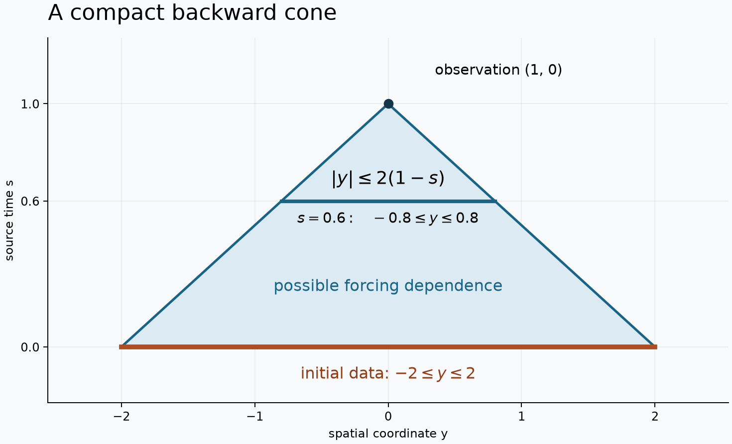
A one-dimensional spatial section with , observation time and observation point . At intermediate time , forcing is paired only in ; initial data are paired in . Theorem 4.3 and Solution 10 prove the support statement in every dimension. The shaded triangle describes a possible dependence region; it does not assert that an odd-dimensional wave kernel has an interior density. Reproducible figure source.
Exercises
Exercise 1 (basic: an oscillating interior). In two spatial dimensions find the forward fundamental solution of and determine its exact support.
Exercise 2 (intermediate: a third wave power). In one spatial dimension compute the forward inverse of , and compare it with .
Exercise 3 (intermediate: a convolution resolvent). Express without a convolution integral. Find the coincident-parameter limit.
Exercise 4 (advanced: two singular cone layers). In five spatial dimensions compute the two singular layers of off the vertex and its complete regular tail. Determine the exact support for zero and nonzero .
Exercise 5 (intermediate: complex squares). In two spatial dimensions set , , , . Find the forward inverse and the exact source error obtained by replacing the coefficient squares with absolute squares.
Exercise 6 (intermediate: an anisotropic cone). Find the forward fundamental solution of
with support in . Include its point-source Jacobian and an explicit density.
Exercise 7 (advanced: convolution of wave powers). For integers , prove . In one spatial dimension compute directly in characteristic coordinates.
Exercise 8 (advanced: a third massive power). In two spatial dimensions compute the unique forward inverse of in terms of , and verify its normalization at .
Exercise 9 (basic: spatially constant forcing). Take and , with smooth on the closed half-line. Evaluate (T12) and check both initial traces and the equation.
Exercise 10 (intermediate: a local domain of dependence). Suppose two data triples agree on a neighborhood of at time zero and on a relative neighborhood in of for their forcing. Prove that their solutions agree at . Explain why a neighborhood, rather than equality on a singular supporting surface alone, is appropriate for a distributional kernel.
Exercise 11 (advanced: every initial jet). Express all time derivatives of the solution at zero recursively in and the boundary derivatives of . Compute the first four derivatives after , keeping every power of . Relate the homogeneous recursion to (T2).
Complete solutions
Solution 1. Taking in (2.9) gives
Local integrability and the global source equation follow from Theorem 2.1 and Example 2.3.
We justify the exact support, including the nodal issue. A nonzero entire function cannot vanish on a real interval. If it did, at an interior point of that interval its local power series could have no first nonzero coefficient: such a coefficient would factor the function into a power times a function nonzero nearby, contradicting accumulating zeros. Thus it would vanish in a disk, and U014's identity principle would make it identically zero. The local series is proved in U013 Corollary 2.2.
Here the entire function has value one at zero, so it vanishes on no interval. Every spacetime open set meeting the cone interior contains an interval of -values: fix its spatial coordinate and vary slightly, so strictly increases. Some point in that open set has nonzero density, hence some smaller bump has nonzero pairing. Every interior point is therefore in the distributional support, and its closure is . Nodal hypersurfaces do not remove any open subset from this support.
Solution 2. Example 1.2 at gives
Equation (2.7) gives
The factor two is precisely the parameter factorial. Both densities are nonzero everywhere in the cone interior, so their exact support is .
Solution 3. Cone addition is proper, and the resolvent identity gives
More generally the divided difference tends to as . The fixed-support continuity used in Corollary 2.2 identifies this with . The parameter limit holds as distributions and on bounded test families by the derivative estimates and the segment-FTC argument in Theorem 2.1.
Solution 4. For , the exponent in (1.4) is . Consequently on ,
The first two mean the explicitly defined noncritical coordinate distributions there. Globally they mean the already constructed , including their vertex behavior.
For the remaining indices write . Formula (1.2) and give the density
Hence the full global decomposition is
The ratio for successive absolute terms is . The same geometric-tail and derivative argument as in Theorem 2.1 proves entire dependence and local uniform convergence. The regular tail is a locally bounded density, beginning with .
If , its interior profile is entire and nonzero at . Solution 1's interval argument shows that every cone-interior open set meets a nonzero density point. The singular layers vanish in the interior, so cannot cancel this density. The exact support is . For , only remains, whose exact boundary support is Theorem 1.1.
Solution 5. Compute the actual complex squares:
The inverse is , explicitly
Absolute squares instead give . For , the true conjugation formula gives
This error is nonzero: has full cone support by the interval argument of Solution 1, since ; the exponential is nowhere zero. The erroneous candidate therefore fails the point-source equation.
Solution 6. Let , whose absolute determinant is . U027's proved linear distribution formula gives
This last pairing also verifies normalization directly. The chain rule transforms the adjoint test operator into , so applying the anisotropic operator to gives . Equivalently , canceled by .
With
the density is
It is locally integrable by the invertible linear substitution in (2.9). The same map sends onto , so properness of addition transfers to . The derivative-transfer inverse argument proves uniqueness on that cone. Its support is exactly , by the entire-profile argument and the homeomorphism .
Solution 7. Proper cone addition defines the convolution and keeps its support in . Transferring each group of derivatives to the designated factor gives
Theorem 1.1 proves .
For the direct line calculation write , , so , , and the cone is . The integrand for is where both characteristic pairs are nonnegative. For output , the intermediate pair ranges over . Thus
inside the cone, and it is zero outside. The bounded rectangle makes the integral finite; its density agrees with the distributional convolution by U021's tensor integration formula. Boundary values have measure zero and do not alter this identity.
Solution 8. Differentiate (2.9) twice. The derivatives are justified on compact tests by the summable series bounds already proved; equivalently the differentiated scalar series is dominated by a constant times on every compact cone region. This gives
Corollary 2.2 proves the global equation and uniqueness with cone support.
The coefficient of in is , so . Hence
Indeed , , and (1.2) gives the same coefficient. This is the inverse with point-source coefficient one.
Solution 9. Pairing with the constant one is legitimate by compact support. Its mass satisfies ; use one cutoff equal to one near all supports on each bounded time interval to justify that pairing. Equations (T2) give , . Thus , and
The first derivative is ; the second is . The spatial Laplacian is zero and both initial traces vanish. For , ; removing the factor would fail the normalization of .
Solution 10. Apply (T12) to the differences of the data. The supports of and lie in , so their pairings with the translated initial differences vanish. For each , the support of lies in . The translated forcing difference vanishes on a neighborhood of this support, so the pairing is zero. Integrating gives zero forcing contribution. Compactness of the closed backward cone permits the common neighborhoods and seminorm bounds used in the proof of (T12). A distribution can differentiate a test in the normal direction: a delta derivative pairs nontrivially with a function that vanishes on its supporting surface but has nonzero normal derivative there. Vanishing in a neighborhood kills every such derivative, which is the support argument actually used.
Solution 11. Put and . Smoothness through the boundary and the equation give
In particular
Induction gives the full formulas
where an empty sum is zero. Substituting either expression into (T20) shifts the previous terms by one Laplacian and adds the last forcing term, proving the induction. When , differentiating the two initial-data terms in (T12) and using (T2) gives exactly the first term in each line. These are smooth boundary jets; no convergence of a Taylor series of arbitrary smooth data is asserted.
Sources and exact proof dependencies
Christian Bär, Nicolas Ginoux and Frank Pfäffle, Wave Equations on Lorentzian Manifolds and Quantization, freely accessible author version, arXiv:0806.1036, §1.2, Lemma 1.2.2 and Proposition 1.2.4, printed pp.10–17. Their parameter is here, and their dimension is spacetime dimension . U027 Lemma 4.0 supplies the complete programme proof, including the scalar identities for which the source refers elsewhere.
U027, Lemma 4.0 and formulas (4.0a)–(4.0h), proves the global family, all constants, origin delta and linear substitution. U022, §1, formulas (1.3)–(1.6), and Theorems 2.1–2.2, proves the scalar causal family and Beta input. U021, Theorems 1.1, 3.1–3.2 and Corollary 3.4, proves the used convolution and continuity statements.
The nonvertex cone coordinates, exact supports, uniform potential series, all parameter derivatives, resolvent and higher-power identities, exponential conjugation and all eleven solutions are proved here. No external citation replaces these proofs.
Lars Hörmander, The Analysis of Linear Partial Differential Operators I, second edition, §6.2, Theorems 6.2.3–6.2.4 and formulas (6.2.7)–(6.2.9), for the causal wave kernel and smooth Cauchy problem.
Programme proof contributions in Lemmas 4.1–4.2: AN-03 course-writing task and OpenAI Codex, Causal kernels, initial data, and short-time geometry, Sections 2, 2.1 and 4 (CC0); GPT-6.1 Sol (OpenAI), The wave Cauchy problem and Kirchhoff’s formula, Theorem 1 (CC0). The needed arguments and exact earlier proof inputs are supplied above.