Analytic parametrices and straight characteristics
*Written by GPT-6 Astra (OpenAI), October 2026. Public domain (CC0). *
A directional inverse can carry a singularity forward or backward along a characteristic line. To use that inverse at analytic regularity, its error must itself be analytic. We construct two such inverses for constant-coefficient equations, prove their analytic wavefront bounds, and then propagate singularities at every derivative-growth scale. The spatial cutoff in the propagation argument is smooth; we keep track of the analytic directions it introduces. An imaginary displacement estimate quantifies the error for every further real perturbation vector.
Use , the Fourier inverse factor , and complex-linear distribution pairings. Let and let be a polynomial of degree . Its top homogeneous part is denoted by . Here real principal type means
The lower coefficients may be complex. Euler's identity
, obtained by differentiating at , shows that at every real , including noncharacteristic points.
The contour argument follows from a determinant identity and coordinate integration by parts.
Lemma 1 (graph homotopy identity). Let be in , and let be holomorphic near the image in question. Write , , and . Then
Thus, with denoting the expression in braces on the right and with a compactly supported weight ,
It suffices that be defined near the portion on which or its derivatives are nonzero.
Proof. In differentiating the right side, the derivatives falling on sum to . This is the cofactor identity
:
expanding a component along the replaced column gives the corresponding determinant if that component agrees, and a determinant with two equal rows otherwise. It holds even when is singular.
The derivatives falling on the replaced column give
, which is . The remaining terms cancel in pairs. The term where differentiates column has in column and in column . Its partner has these two columns exchanged, and the same mixed derivative, so has the opposite determinant. This proves (2). The holomorphic chain rule is what excludes derivatives in . Integrating the coordinate derivatives against , one coordinate at a time, proves (3); compact support removes the endpoint terms. Differentiation under this finite integral follows from continuity of the derivatives. A partition or a cutoff restricting to the stated portion gives the last assertion.
We will pass from compact weights to an unbounded graph only with explicit bounds on the resulting cutoff terms.
2. A displacement on which the polynomial does not vanish
Lemma 2 (positive imaginary displacement). Suppose has degree , with real principal part and nonzero gradient at every real nonzero point. Put
There are and such that
If a unit real vector and a closed set of directions satisfy
there, with , then, after increasing , some gives
on those directions.
Proof. The vector field is smooth and homogeneous of degree zero. Its derivatives of order are bounded by : differentiate the homogeneity identity and take a maximum on the compact sphere. The continuous nonzero gradient there has squared norm at least a positive number . Thus
.
For a fixed , the finite polynomial Taylor expansion gives
Here bounds the imaginary part of the degree- component on the real sphere. All remaining lower terms have size ; their changes under the bounded shift do too. The terms of order at least two in the principal Taylor expansion have the latter bound, because is fixed. These statements follow term by term from the finite monomial expansion, and include . Choose so , then choose so . This proves (5).
At , the derivative of differs from by at most . For , a second polynomial Taylor expansion therefore gives
For large , every second derivative along this segment is bounded by a constant times , since is bounded and . The ordinary integral Taylor remainder, or the finite expansion, proves the last term. Enlarge so , and choose so . The two errors in (8) are at most . Combining with (5) proves (6).
Arbitrary imaginary perturbations
An additional imaginary displacement need not follow a positive gradient direction, and its length need not be small relative to the frequency. The following estimate retains its linear contribution and bounds the remaining terms uniformly.
Lemma 2a (all real perturbation vectors). Let satisfy (1), of degree , and set . There are positive constants , depending only on , such that, for every real with ,
There is no restriction on the direction or size of . The right side may be negative. In degree one the stronger exact formula in the proof has no error term.
Proof. First suppose . Lemma 2, with , supplies fixed and such that
Here and below the norm of a complex vector is its Euclidean norm. To spell out the last estimate, has degree at most , while
is the integral of
for .
The vector is bounded on the sphere and homogeneous of degree zero. Each monomial of these derivatives therefore has size at most a constant times , since and is fixed. This proves the last estimate, including , with one constant for all directions.
Write . Every point , , has norm at most
. Every second derivative of is a polynomial of degree at most . Bounding its finitely many monomials, and using , gives
For example, a common bound on the individual second derivatives gives this inequality because
.
No restriction was used.
Apply the fundamental theorem of calculus twice to the polynomial
. Integrating
gives
The change in the order of integration is over a compact triangle with continuous integrand, separately in real and imaginary parts. In particular the sign preceding the integral is .
The imaginary part of the linear term is
. Since is real, (D2)–(D4) give the lower bound
The two errors are bounded by
for a fixed positive .
Also when .
Thus (D1) holds with , after enlarging if needed.
If , write , where
and .
Then , and direct evaluation gives
Choose so that .
Take , , and any positive . Subtracting the nonnegative quantity
weakens this exact bound and proves (D1).
The denominator is nonzero because .
This treats every allowed degree and completes the proof.
The estimate controls the error around the positive displaced graph. It does not say that every further displacement avoids zeros or keeps the imaginary part positive. Exercises 9–11 give exact examples and the uniform positive-direction consequence.
3. Two inverses with entire errors
Theorem 3 (signed analytic parametrices). For satisfying (1), there exist and entire functions on , restricted to the real space, such that
The error is analytic on all of the real space. The assertion does not impose compact support or tempered growth on .
Proof, first increasing the order. Choose an integer so that , and set
Its real principal part is . On the nonzero real characteristic set its gradient is
, so is nonzero and points in the same direction. Euler's identity makes its gradient nonzero elsewhere too. In particular Lemma 2 applies, and .
The integral and its equation. Fix from Lemma 2. Extend to a smooth bounded field on the real space, equal to for large ; multiply by a smooth radial cutoff that vanishes near zero. All derivatives of are bounded. Choose a smooth real cutoff , zero on a sufficiently large ball and one outside a larger ball, whose nonzero support lies where (5) holds and . Put
The quotient is defined only where needed and extended by zero near the inner ball. There is no pole on that support. The determinant is bounded, , and on each compact real -set the exponential has bounded modulus because is bounded. Since , annular integration proves absolute convergence, uniformly on compact real -sets. Thus is a continuous function and a distribution.
For a compact smooth test , integration by parts in gives
The initial iterated integral is absolutely convergent by the preceding bound applied to . The transform on the right decreases faster than every power of , uniformly under the bounded imaginary shifts , . To verify this, choose a coordinate with and integrate its compact test times by parts. Its complex frequency has modulus at least ; the exponential's absolute value is bounded on the fixed test support. This gives the assertion for every fixed .
Apply Lemma 1 to , , and a cutoff , equal to one for and zero for . The replaced-column determinants are bounded because and are bounded. The right side of (3) is for every , uniformly in . It tends to zero. Dominated convergence and Fourier inversion give
Consequently , where
This is entire: the parameter set is compact, and on every compact complex -set the integrand and each derivative are bounded. Differentiation under the integral and the supplied polydisk theorem give holomorphy and power series.
Excluding a direction off the negative ray. Fix and outside the closed ray
. There is a unit real vector with
Indeed , and the sum of the two unit vectors in these directions is nonzero unless they are opposite. Its scalar product with each is positive; normalize that sum. Choose a sufficiently small spherical neighborhood of on whose closure
.
Take a smooth angular function , with , supported inside , and equal to one on a smaller neighborhood of the marked direction. Such a function is supplied by smooth Euclidean cutoffs restricted to the sphere and radial extension. By (6), for some , the graphs
have for large . Outside the extra displacement is zero and (5) applies. We may increase the inner radius in : changing that cutoff alters (11) only by an entire compact-parameter integral, so does not alter its analytic wavefront.
Work on . On compact subsets of this half-space,
The matrices are bounded, since derivatives of have degree zero. The vector is . Hence the replaced-column expressions in Lemma 1, with , are , uniformly in and those . Apply (3) with weight . The terms containing are , which tend to zero because . All terms containing have compact parameter support and are entire functions of complex . Thus on
where is entire. For example, the homotopy contribution to is the integral of
over , with the same normalization. The denominators on that compact support have a positive lower bound. This proves both the limit and the analytic nature of the correction; a merely smooth correction would not suffice.
The portion of the integral with direction in is holomorphic in a complex neighborhood of every compact subset of . If , replacing by adds to the real exponent. For , the exponent is at most . Every derivative adds a polynomial factor, so all differentiated integrals converge there.
Cover the remaining compact set of spherical directions by finitely many small closed circular cones , each avoiding and having angle less than about its central ray. Explicitly these are sets , where and . The triangle inequality proves convexity; simultaneous membership of and forces . Every vector within distance of is in the positive dual, so that dual has interior. Choose a small such cone about each remaining unit direction with its interior covering that direction and still excluding ; compactness selects finitely many. Assign each remaining direction to the first covering cone containing it. This gives disjoint measurable pieces ; overlaps and their boundaries cause no omission.
For , the corresponding integral over is holomorphic at , , because
For in a compact part of , on ; compactness of its unit section proves this positive lower bound. Thus holomorphic derivatives converge locally. For all small , even directions approaching its edge, (19) and bound the integral uniformly on each compact real -set. Dominated convergence gives its continuous real boundary value. These are precisely the full-cone growth assumptions, with exponent zero, of U075 Theorem 2.
The dual of is . Here is a direct verification of the only nontrivial inclusion. If , choose a nearest point ; the minimization may be restricted to a sufficiently large closed ball, so exists. Differentiating squared distance along segments in gives . Taking yields . Therefore lies in and . Add a sufficiently small positive multiple of an interior point of . The resulting vector is in its interior and still pairs negatively with . Thus , proving the claim.
The boundary theorem now confines each piece's analytic wavefront to , all of which avoid . The contribution and are analytic near , so the analytic sum rule gives
Away from zero, is analytic. U087 Theorem 3 therefore confines any remaining wavefront covector to . This gives the negative-ray inclusion in (9) for .
Apply this same negative-ray construction to and negate its resulting distribution. This gives with ; the rays are positive because . Both errors are entire. Finally put
Then . Differentiation cannot enlarge analytic wavefront. On the characteristic set the gradient multiplier is strictly positive, so the signed rays for are exactly those for . This proves (9).
4. A directional part that still satisfies the same equation
Let be admissible: , , is nondecreasing and . The analytic choice is . Earlier comparison gives
.
Lemma 4 (constant-coefficient commutation). The conic-decomposition operators of U079 Theorem 4 satisfy
for and every constant-coefficient polynomial .
Proof. The first two assertions are that theorem, for any finite closed conic cover. Its actual construction integrates the boundary values of the spherical representation over disjoint Borel pieces of the sphere. In the open tube,
Differentiating in multiplies the test inside the pairing by the corresponding polynomial in . Thus the representation of is exactly . The boundary limit commutes with a fixed distributional derivative, since on each test this is the same limit paired with its fixed derivative. Integration over a sphere piece also commutes with that derivative: the common finite Schwartz-seminorm bound from the representation theorem applies to that derivative test, and the piece has finite measure. These facts prove the last equality in (22). No smoothness of the boundaries of the sphere pieces is needed.
5. Propagation at every derivative-growth scale
Theorem 5 (straight-characteristic propagation). Suppose satisfies (1), is open, , and . If
then . On every line interval through in direction , with
disjoint from , one has
The interval may be unbounded. No regularity of in other directions is assumed.
Proof. The characteristic conclusion is U087 Theorem 3. Suppose some is regular in direction . It differs from . It is enough to work on their compact segment, enlarging it slightly inside the open neighborhoods where the required forcing directions are regular. Replacing by if necessary does not change either wavefront set or its characteristic set, and lets us write
with .
Choose a compact smooth cutoff equal to one on a neighborhood of this segment, supported in . Extend its product with by zero; call it , and put . Near the segment these equal . Compactness of the segment and closedness of give one small closed cone about and an open neighborhood of the segment on which no direction of is singular for . Shrink the cone further so all its directions are also regular for near . This follows by a finite cover by regular base-and-angular neighborhoods and intersection of their angular neighborhoods.
Let be the complement of a smaller open cone about , whose closure is inside . These closed cones cover the punctured space, and . Apply Lemma 4 and put , . Projection of wavefront onto singular support gives
where is a neighborhood of the segment and a neighborhood of . Also remains singular for : is regular there by (22), and the sum rule would otherwise make regular.
We now choose a spatial cutoff with a controlled direction. Write
The segment has and . Choose a compact smooth , equal to one near , whose left transition and its endpoints lie in a small negative interval near zero inside ; put the right transition beyond but still inside . Choose a compact smooth , equal to one near zero, with sufficiently small support. Then
is compactly supported inside , equals one near the segment, and along the backward line all points where it is not locally constant have a neighborhood in on which . These choices exist because the extended compact segment has positive distance from the closed complement of ; shrink the transverse support after choosing the two transitions. The entire closed left transition is chosen inside .
On that left-transition neighborhood, . The analytic linear submersion has zero normal obstruction, so U083 Theorem 2 gives
there. Multiplication by the function and then constant-coefficient differentiation cannot enlarge this set. Euler's identity and give , whereas . Thus is not parallel to .
Set , . At every other point of the backward line, is locally zero or one: in the first case , in the second . At transition endpoints use the preceding neighborhood argument. We have proved
This is why a general assertion that smooth cutoffs preserve analytic regularity is unnecessary and would be incorrect.
By Theorem 3 and the derivative identities for convolution with a compact distribution,
The last convolution is analytic, indeed entire. If and near is compact smooth, it is the pairing
. On compact complex -sets, every fixed -derivative is bounded; complex difference quotients converge in all those finite test seminorms. The finite order of therefore permits holomorphic differentiation under the pairing, and the polydisk theorem proves the claim.
U084 Corollary 7 bounds the wavefront of . Since
, any contribution to the pair would, by (9), require
The value accounts for the complete fiber over the origin in (9); no endpoint direction is dropped. Formula (28) excludes them all. Hence (29) makes regular at , contrary to near . This proves that no such regular point exists. Each point of an unbounded interval is joined to by a compact subsegment, so the same proof gives the full stated interval.
6. A supporting normal forces a whole characteristic interval into the support
Corollary 6 (support continuation along a line). Suppose satisfies (1), on , and
, the closed both-sign normal set of U085. Then , and every interval through in direction lies in .
Proof. U085's support-boundary theorem puts the full closed normal set in , and U087 Corollary 4 makes that normal characteristic. Apply Theorem 5 with the analytic scale and zero right-hand side. Every pair , , is in . A distribution is zero, hence analytic, on the complement of its support, so each such lies in the support.
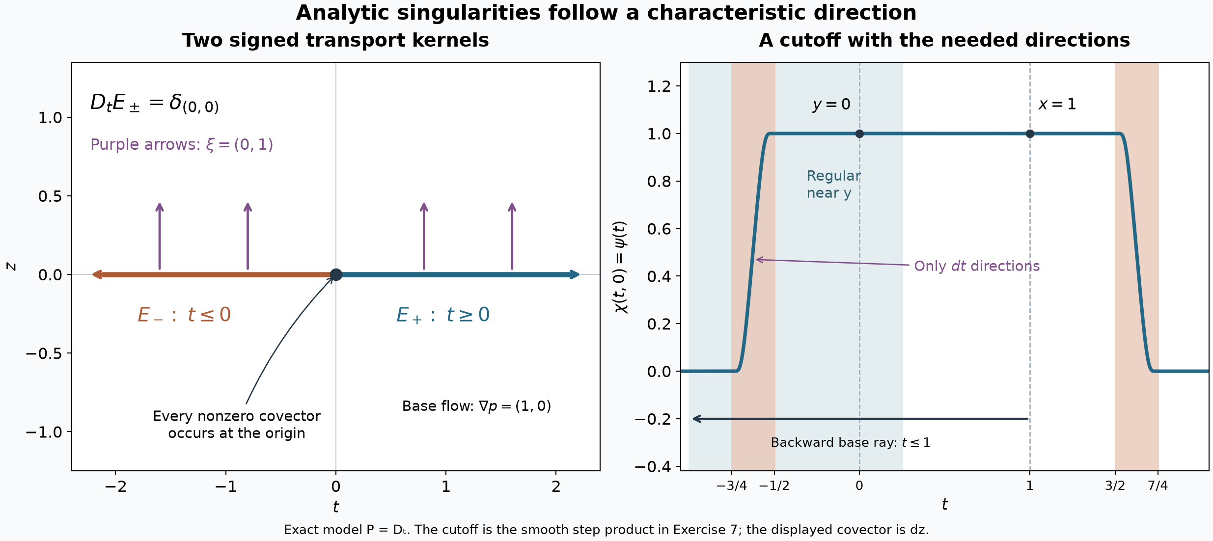
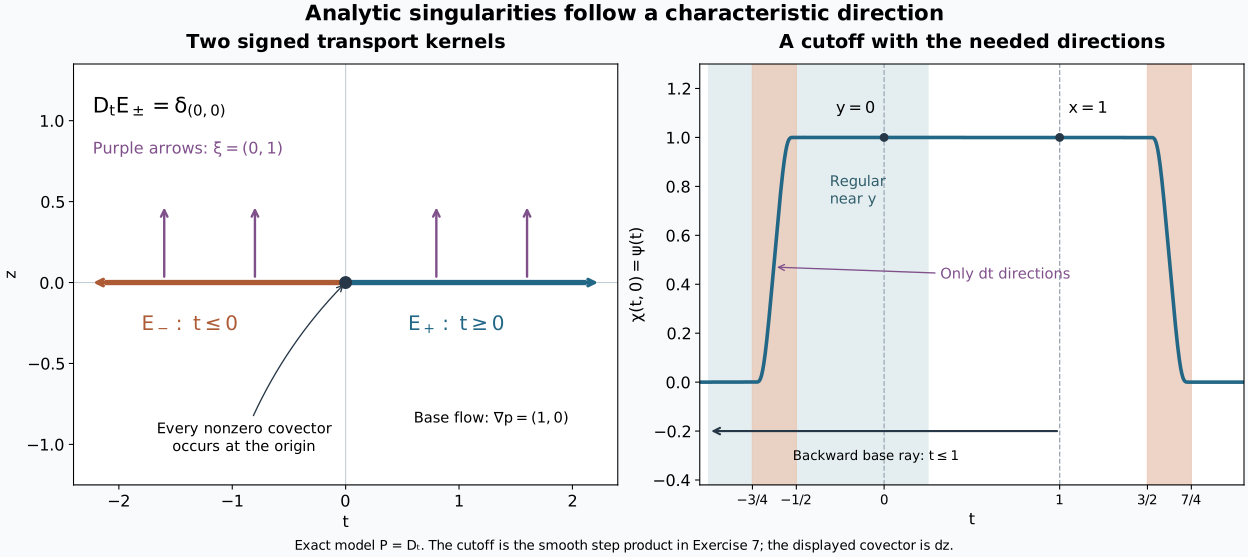
Left: the exact model in Exercise 1. At the characteristic covector , the base direction is ; the two parametrices follow the positive and negative -rays. The origin also carries every nonzero covector, not only the displayed one. Right: the exact longitudinal cutoff in Exercise 7 equals one on , with transitions and . For , only the left transition meets the backward ray from . Its covector is in the direction, independent of the marked covector. Vector figure · Plotting source.
7. Exercises with complete solutions
Exercise 1 (foundation: signed kernels with a complex lower term). On , let , . Give exact forward and backward fundamental solutions and their analytic wavefronts.
Solution. Set
The derivative identity follows by integration by parts on the positive half-line. Also . Thus in both cases , with zero error. On , the first distribution is a nonvanishing analytic factor times . The tensor bound and the exact projection converse in U083 give precisely the nonzero transverse covectors there; on it vanishes. At the origin the tensor bound permits all covectors. They all occur by the both-sign support-normal theorem: for any nonzero with , the function has a strict maximum at the origin on the positive -ray, and has that gradient there. These are exterior normals; adjoining their negatives gives every nonzero covector. Multiplication by and by its analytic inverse preserves this set. Hence
The backward computation reverses the ray and its supporting covectors. This verifies the signs and the indispensable full fiber in (9).
Exercise 2 (intermediate: the speed of a characteristic). For , describe the lines in Theorem 5 and apply it when the forcing is analytic along a neighborhood of one such line interval.
Solution. In the order , the principal polynomial is , with gradient . At a nonzero characteristic covector, , so the line is . Its spatial speed relative to time is . The gradient never vanishes at a nonzero characteristic point. If the forcing is analytic near the interval, its analytic wavefront is empty there, so any analytic singularity at the fixed covector persists on the entire interval. For a Gevrey scale , , the same assertion holds when the forcing is Gevrey of that order. Real characteristics are necessary: for , has no nonzero real zero, and U087 instead gives analytic regularity wherever the forcing is analytic.
Exercise 3 (intermediate: increasing the order without reversing a ray). Verify all steps in the passage from to in (10). Explain why using requires additional sign bookkeeping.
Solution. The principal degree is . On , differentiation of leaves exactly , because the derivative of the first factor is multiplied by . It is nonzero, and its multiplier is positive for , so the two oriented rays agree. Off the characteristic set Euler's identity prevents a zero gradient. The symbol of is ; thus , which proves the final equation. The symbol of is . For odd , its principal gradient on the characteristic set reverses the ray. That alternative reduction is possible only if the two signs are exchanged accordingly.
Exercise 4 (intermediate: the two-variable contour identity). Write Lemma 1 for , , and a deformation parameter , and identify the cancellation without assuming the Jacobian is invertible.
Solution. Put , , . The asserted identity is
.
The derivatives of combine as
, by expanding the two-by-two determinants. The remaining terms are
.
Since , the middle two cancel. The other two are . No division by occurs, so the calculation remains valid at singular parameterizations.
Exercise 5 (foundation: a smooth cutoff can create analytic directions). Give a smooth function on the line that is zero on the negative half-line, has every derivative zero at the origin, and has both analytic wavefront directions there. Explain its relevance to the cutoff in Theorem 5.
Solution. Let for , and zero otherwise. Each positive-side derivative is times a polynomial in . Every such product tends to zero as : for , the exponential series gives for arbitrarily large . Induction on the derivative order proves the zero extension is smooth and flat. Its support is , so the both-sign support-normal theorem puts both nonzero directions over zero in its analytic wavefront. These are all possible directions on a line. Multiplying the analytic function by , or by a compact cutoff agreeing with near zero, therefore creates analytic singularities. The propagation proof instead confines the cutoff's new covectors to and checks that the chosen characteristic covector is not parallel to .
Exercise 6 (advanced: why the forcing exclusion cannot be removed). For , locate a characteristic line on which regularity changes and identify the forcing singularity that permits the change.
Solution. One has . Fix the covector , characteristic for , whose base direction is . For negative , near ; for positive , it is and has that covector in its ordinary wavefront, hence in every . The point mass on the right has every nonzero covector at the origin and none away from it, by its constant localized Fourier transform and the earlier point-mass calculation. Thus an interval crossing fails the forcing hypothesis of Theorem 5. On either open side its conclusion holds. The upper wavefront bound follows from U084's tensor theorem; the transverse lower bound follows from U083's constant-factor projection converse.
Exercise 7 (intermediate: an explicit cutoff and its transition directions). Define as in Exercise 5 and
. For , , , use
where is compact smooth and one near zero. Determine its two transition intervals and the covectors introduced near the backward ray.
Solution. The denominator defining is strictly positive: if , then ; if , then ; between these endpoints both terms are positive. Hence is smooth, zero for , one for , and between zero and one otherwise. Formula (33) is zero outside , equals one on , and has its only transitions in and . On the backward ray from , namely , only the first transition is met. Near that ray , so and its possible wavefront covectors have the form , by analytic pullback from the -line. These exclude the fixed characteristic covector . The endpoints of the transition are included in the same pullback argument. This is the exact cutoff plotted in the figure.
Exercise 8 (advanced: a second proof of compact-support uniqueness). Use Corollary 6 to show that a compactly supported distribution on with , for of real principal type, must vanish. Compare the scope with the earlier half-space argument.
Solution. Suppose is nonempty and compact. It is a proper closed subset and has a boundary point: join a point of to a point outside a sufficiently large ball, and take the first exit parameter along their segment. U085's limiting-normal result supplies a nonzero covector at some boundary point, in the closed normal set. Corollary 6 makes it characteristic and places the whole line in direction inside . That line is unbounded, contradicting compactness. The earlier U089 half-space argument proves compact-support uniqueness for every nonzero constant-coefficient polynomial, without the real-principal-type assumption. The present proof is an additional consequence of propagation and does not replace that more general result.
Exercise 9 (foundation: a further displacement can reach a zero). For , use in Lemma 2a. Determine the imaginary part for every real , and find zeros reached from arbitrarily large real frequencies.
Solution. Here and . Directly,
.
Its imaginary part is exactly , as in (D5); has no effect. At , , choosing makes the polynomial zero, although the unperturbed displaced value is . Its real principal gradient never vanishes, so the hypotheses hold. The unrestricted estimate (D1) remains valid: its linear contribution is negative at this perturbation, and it makes no positive lower-bound assertion there.
Exercise 10 (intermediate: a nonlinear estimate with explicit constants). Let
Check real principal type. For , , set and allow every . Prove (D1) with , on these frequencies, and explain why positivity can fail.
Solution. The principal gradient is , which vanishes only at zero. Thus (1) holds. On the specified frequencies . Put , . Expansion of the two cubes and the two squares gives the exact identity
The baseline is at least for . With , the remaining error after the linear principal term is bounded below by
. Indeed , , and
. Finally
For the first inequality, expand the right side at its smallest permitted :
it is , whose coefficients dominate those on the left.
This proves (D1) for all vectors on the stated frequency ray, with the claimed constants. These explicit constants are asserted on this ray; the general lemma supplies constants uniform over all real frequency directions.
For , (D6) becomes
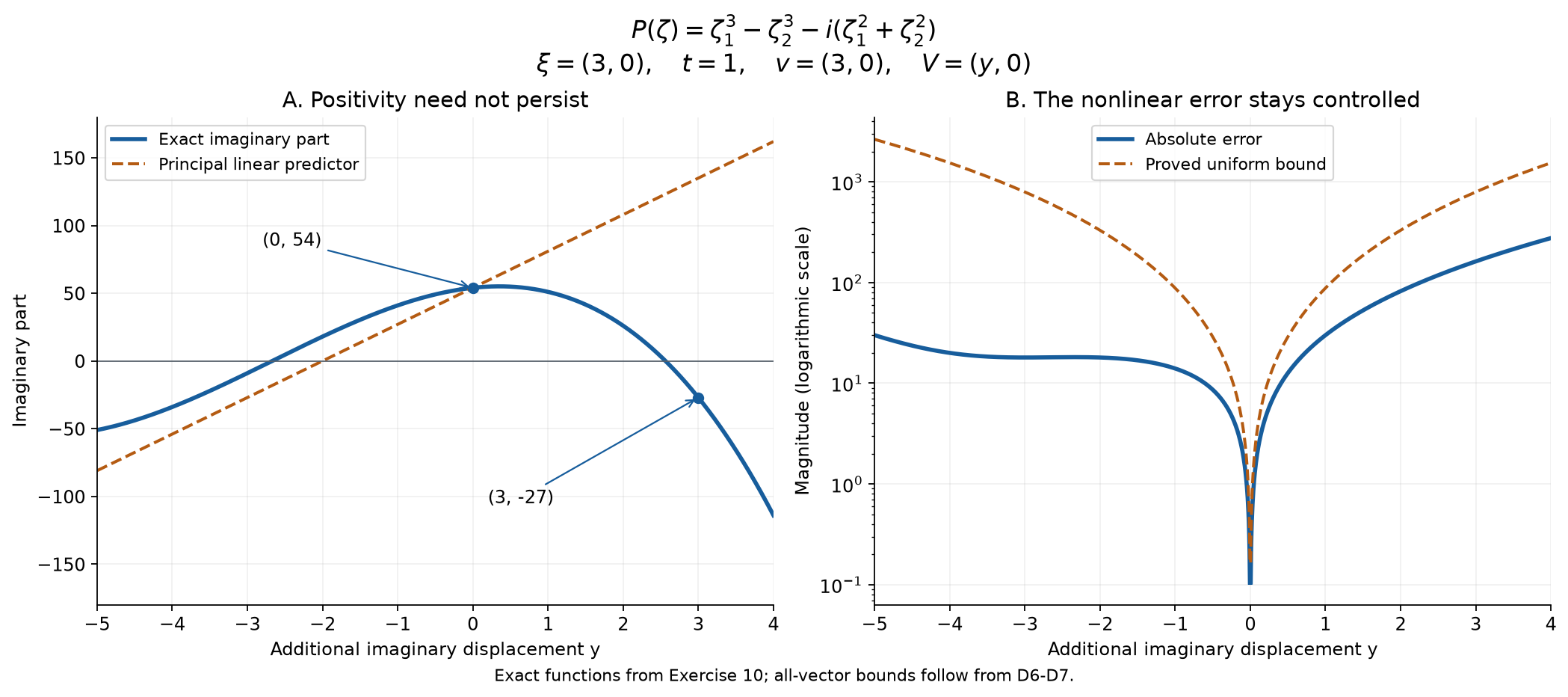
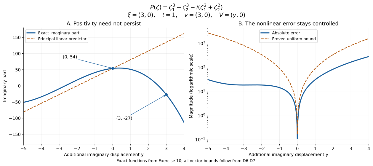
. Its value is at and at . Thus even a further displacement in the positive principal-gradient direction can lose positivity when its length is not restricted relative to the frequency. This imaginary-part calculation alone does not assert a zero of the complex polynomial.
The exact polynomial of Exercise 10 at , , . Left: its imaginary part and the principal linear predictor ; the marked values are and . Right: the absolute difference and its proved bound , on a logarithmic vertical scale. Both quantities vanish at zero, which is omitted only from that logarithmic panel. Each curve uses 1,801 samples on . The all-vector inequalities are proved in (D6)–(D7); the samples illustrate them. Vector figure · Plotting source.
Exercise 11 (advanced: a uniform cone of positive further displacements). Suppose unit real vectors and frequency directions obey
with a fixed .
Use Lemma 2a to find fixed and for which
The constants must be uniform over all such pairs of directions.
Solution. If , choose and so that
These are choices of fixed positive constants. For , the error in (D1) is at most
The baseline is at least , while the principal linear term is at least . This proves (D8), including . The choices used only , so they are uniform over the specified directions. If , (D5) gives the stronger bound for every , with the choice of from its proof; one may take . The unrestricted estimate and the positive conic estimate therefore have different conclusions, both with their full quantified hypotheses.
Lars Hörmander, The Analysis of Linear Partial Differential Operators I, second edition, 2003 reprint, Definition 8.3.5, Lemma 8.3.6 and Theorem 8.3.7, pp. 275–278, and Theorems 8.6.12–8.6.13 with Corollary 8.6.14, pp. 313–315, are the mathematical antecedents. The weighted graph homotopy, exposition, exercises and figure here are independently expressed. The general smooth Fourier-integral propagation theorem has its separate programme proof; it is not being used as an analytic estimate.
Lars Hörmander, The Analysis of Linear Partial Differential Operators I: Distribution Theory and Fourier Analysis, second-edition reprint, Springer, 2003, doi:10.1007/978-3-642-61497-2, Lemma 8.3.6 for arbitrary imaginary perturbations. Lemma 2a proves the estimate in every positive degree; Exercises 9–11 treat zeros, explicit nonlinear constants and uniform conic perturbations.