Tangent support and analytic directions

Exposition, proofs and exercises: GPT-6 Astra (OpenAI), October 2026. CC0.

There are two different geometries at a singular point. The support has directions in physical space along which it approaches the point. The analytic wavefront has a closed set of directions in the cotangent fiber. A normal to this latter set must point along the physical tangent cone, with both signs. This relation propagates analytic regularity through convex regions of a fiber and explains why analytic Cauchy data control all normal frequencies near a noncharacteristic boundary. An explicit smooth counterexample shows the force of the analytic hypothesis.

Pairings are complex-linear, , and the Fourier sign is . A Euclidean scalar product identifies vectors and covectors when distances or normals are taken inside one fiber. Analytic changes of coordinates retain the intrinsic tangent and cotangent meanings.

The Gaussian transform of a compact hyperfunction, represented by an analytic functional, is $G_\lambda u(z)=u_y\!\left(e^{-\lambda(z-y)^2/2}\right), \qquad \lambda>0,\quad z\in\mathbb C^n, \qquad (z-y)^2=\sum_{j=1}^n(z_j-y_j)^2. \tag{T1}$ The distance estimate, local representative independence and exact exponential criterion for analytic wavefronts are Gaussian windows and analytic directions, Theorems 1 and 4 and Corollary 5. The finite closed-cone decomposition and its holomorphic sides are Directional splitting and holomorphic compatibility, Lemma 1 and Theorem 2. Analyticity when the whole fiber is regular, and agreement with the distributional analytic wavefront, are Holomorphic boundary values without growth bounds, Theorem 3; its Theorem 7 gives the converse holomorphic wedge representation used in Theorem 2 below. Compact representatives and localization are proved in Hyperfunctions from local analytic sources.

The geometry of supporting functions and their strict quadratic replacements is Both analytic directions at support boundaries, (1)–(4); its Theorem 4 proves the convex contact assertion used below. The maximum principle is Positive derivatives and canonical representatives, Theorem 3.4, and subharmonicity of the logarithm of a holomorphic function is Compactness and complex-line positivity, Proposition 3.2. Finite-dimensional compactness, derivatives, integration and limiting operations use the supplied scalar and integration foundations.

Distances between dual cones

For a closed convex cone , put $C^\circ=\{r:r\cdot q\le0\text{ for every }q\in C\}. \tag{T2}$

Lemma 1 (orthogonal cone projections). For every there is a unique nearest point . If , then is the nearest point of to , , and $d(\eta,C)^2+d(\eta,C^\circ)^2=|\eta|^2. \tag{T3}$ Consequently, if is a closed pointed convex cone and , where , then $d(\eta,G)^2=|\eta|^2-d(\eta,-\Gamma)^2. \tag{T4}$

Proof. Since , a minimizing sequence can be confined to a fixed closed ball: a point with cannot improve the competitor . Compactness and closedness give a minimizer. Strict convexity of squared distance gives uniqueness, since the midpoint of two distinct minimizers in would be closer.

Differentiate the squared distance along the segment from to : $(\eta-p)\cdot(q-p)\le0. \tag{T5}$ The choices give ; (T5) then gives . For , one has . Expanding proves that minimizes distance to in . Orthogonality proves (T3).

For the last assertion, the cone-duality identities proved in Lemma 3 of the directional-splitting lesson give and . Distance to an open set equals distance to its closure. Apply (T3) with .

Gaussian growth after magnifying a point

Translate the point under study to . For a compact hyperfunction , let $F=\{\xi\ne0:(0,\xi)\in\operatorname{WF}_A(u)\},\qquad W=F\cup\{0\},\qquad h_W(\eta)=\frac{|\eta|^2-d(\eta,-W)^2}{2}. \tag{T6}$ The set is a closed cone. Adjoining matters when the fiber is empty: then and . For , write , where . This is composition with for functions, with the usual inverse-Jacobian factor in a distributional pairing.

Theorem 2 (the rescaled growth profile). Let be compact and let be continuous on a neighborhood of , with $\Phi(z)>h_W(\operatorname{Im}z)\qquad(z\in K). \tag{T7}$ There is such that, for every , a constant satisfies $|G_\lambda u_\delta(z)|\le C_\delta e^{\lambda\Phi(z)} \qquad(z\in K,\ \lambda>0). \tag{T8}$ No uniform bound on as is asserted.

Proof. Cover the unit sphere by finitely many small closed spherical caps whose cones are convex and pointed. The closed-cone decomposition gives local summands with wavefronts confined to these cones, and holomorphic representatives on wedges with imaginary direction in . On a smaller common real neighborhood of , choose compact representatives of all the summands. Their sum differs from by a compact hyperfunction zero on .

A cone missing gives a summand whose entire fiber at is regular. That summand is analytic on a smaller neighborhood by the analytic-singular-support theorem, so it has a representative holomorphic on a full small complex tube. There are finitely many such shrinkings. The other cones meet . Let be their union, with adjoined.

We first control how much the cones enlarge . Suppose their angular diameters are at most , and . A nearest point in can be chosen with , using as competitor. If , its cone meets ; at the same radius there is a point with . Thus $0\le d(\eta,-W)-d(\eta,-C)\le2R\varepsilon. \tag{T9}$ If , all summands are analytic and the same conclusion is immediate. Both distances are at most , so their squared difference tends to zero uniformly on bounded -sets as the caps shrink. The positive minimum of on therefore permits a finite decomposition for which $h_C(\operatorname{Im}z)<\Phi(z)\qquad(z\in K). \tag{T10}$

For a singular summand, (T4) gives $\frac12d(\eta,G_j)^2 =\frac{|\eta|^2-d(\eta,-\Gamma_j)^2}{2} \le h_C(\eta). \tag{T11}$ Fix , with . Choose with . Take a small convex approach cone about whose angular closure lies in . The wedge representative has a fixed positive height on this smaller cone over a sufficiently small real base. Intersecting the cone with a small ball gives a convex imaginary set , with . For all sufficiently small , , hence $\frac12d(\operatorname{Im}z,\Omega/\delta)^2 \le \frac12|\operatorname{Im}z-q|^2<\Phi(z) \tag{T12}$ on a neighborhood of . A finite cover of , and the finite number of summands, give one real base and one upper bound for . This argument uses fixed heights only on strict approach cones.

The other hypothesis in the Gaussian carrier estimate is $\Phi(z)> \frac{|\operatorname{Im}z|^2-d(\operatorname{Re}z,\mathbb R^n\setminus(X/\delta))^2}{2}. \tag{T13}$ It holds uniformly on for small , because contains a ball about and the displayed real distance tends to infinity. The carrier estimate now proves (T8) for each singular summand. For an analytic summand take to be a ball about ; its dilates eventually contain every imaginary point in , so the imaginary distance is zero. Here . Finally the zero-on- remainder needs only (T13), by the zero-region part of the same carrier estimate. Sum the finitely many constants.

A subharmonic barrier between two ends of a segment

Lemma 3 (rectangle barrier). Let , and let be subharmonic on , with $v(x+iy)\le(\max(0,-y))^2. \tag{T14}$ Suppose on a collar of the left edge. Set $A(x)=\frac b3\,\frac{\sinh(\pi(a-x)/b)}{\sinh(\pi a/b)}. \tag{T15}$ For and , $v(x+iy)<-A(x)\bigl(2y+A(x)\bigr). \tag{T16}$ The corresponding statement at the right edge follows by .

Proof. Fix , and work on the smaller rectangle . The function $v_d(x+iy)=v(x+iy)-d^2+ bA(x)\sin\!\left(\frac{\pi(y+d)}b\right) \tag{T17}$ is subharmonic, since makes the last term harmonic. Its upper boundary limits are nonpositive. On the bottom and top this follows from (T14) and the vanishing sine. On the right and . On the left the negative collar bound and give a strict negative margin. The maximum principle gives ; the strong maximum principle makes the inequality strict, since a zero maximum in the interior would force constancy, contrary to the left collar.

When , the elementary inequality gives . At the point under consideration choose . Since and , the required sine interval holds, and the last inequality is (T16). Reflection of the real coordinate preserves subharmonicity and the sign of , proving the last assertion.

The tangent cone of support

If belongs to a relatively closed set , define $T_{x_0}S= \left\{\,\lim_{j\to\infty}t_j(x_j-x_0): x_j\in S,\ x_j\to x_0,\ t_j>0,\ t_j\to\infty\,\right\}. \tag{T18}$

Lemma 4 (closure, coordinates and missing directions). This is a closed cone containing . If is a diffeomorphism near , then $T_{\psi(x_0)}\psi(S)=D\psi(x_0)\,T_{x_0}S. \tag{T19}$ If a compact set misses , then $(x_0+\delta B)\cap S=\varnothing \quad\text{for every sufficiently small }\delta>0. \tag{T20}$

Proof. The constant sequence gives , and multiplying the parameters by a positive constant gives conicity. If tends to , choose from the defining sequence for a point and parameter such that and . This diagonal sequence proves closedness.

The differentiability remainder in $\psi(x)-\psi(x_0)=D\psi(x_0)(x-x_0)+o(|x-x_0|)$ vanishes after multiplication by , because is bounded. This gives one inclusion in (T19); the inverse diffeomorphism gives the other.

If (T20) failed, there would be and with . A convergent subsequence in , together with , would give a point of .

Normals to a singular fiber

For a relatively closed , an exterior normal at is a nonzero vector , where is real , , and on near . Interior normals are the negatives of exterior normals. We also allow limits of these pairs inside the punctured fiber.

Theorem 5 (fiber normals lie in both tangent directions). Let be a hyperfunction near , and set $F=\{\xi\ne0:(x_0,\xi)\in\operatorname{WF}_A(u)\}, \qquad T=T_{x_0}(\operatorname{supp}u). \tag{T21}$ For every exterior or interior normal to , and for every limit of such normal vectors with a nonzero limiting base covector, $\nu,\ -\nu\in T. \tag{T22}$ When , there is no normal assertion.

Proof: the normal-distance inequality. Translate to , choose a compact representative, and let have exterior normal . The strict quadratic construction recalled above replaces its witness by a quadratic polynomial with the same differential, , and on nearby . Let near , and write . Shrink the patch so has a positive lower bound.

There is such that $d(\xi+t\nu_\xi,W)\ge t|\nu_\xi| \quad(\xi\in\Sigma\text{ near }\xi_0,\ 0\le t<t_0), \qquad W=F\cup\{0\}. \tag{T23}$ Indeed Taylor's formula, uniformly on a small patch, gives for nearby , since . Hence $|\xi+t\nu_\xi-q|^2 \ge t^2|\nu_\xi|^2+(1-2Ct)|q-\xi|^2. \tag{T24}$ Choose . Points of outside a fixed neighborhood of , including , have a uniformly positive distance from the smaller patch; decreasing makes their distances at least as well. Taking the infimum proves (T23).

Proof: a missing physical direction gives an exponential gap. Suppose one of misses . Lemma 4 gives a fixed ball about that vector, and a slightly larger ball with compact closure disjoint from , on which vanishes for all small . The Gaussian zero-region estimate consequently gives a constant , independent of small , such that $V_\delta(z):=\frac2\lambda \log\frac{|G_\lambda u_\delta(z)|}{C_\delta} \le |\operatorname{Im}z|^2-c \tag{T25}$ near the corresponding endpoint of , for every . To obtain this fixed , use the positive distance from the smaller real ball to the complement of the larger zero ball, and take a strict margin in the carrier estimate.

For any , Theorem 2, on a compact neighborhood of the same segment, gives $V_\delta(z)\le \varepsilon+|\operatorname{Im}z|^2 -d(\operatorname{Im}z,-W)^2. \tag{T26}$ Here is sufficiently small depending on . Increase so that both estimates hold. For fixed , the restriction of to every complex line is subharmonic, or identically .

For real near , near , and , put $H(w)= \frac{V_\delta(x-i\xi-w\nu_\xi)-\varepsilon-|\xi|^2 -2t\,\xi\cdot\nu_\xi}{|\nu_\xi|^2}. \tag{T27}$ The subtracted -term is harmonic. By (T23) for , and by the trivial nonnegativity of distance for , (T26) gives .

Choose small. On a collar of the endpoint or corresponding to the missing direction, (T25) gives . Uniform upper and lower bounds on therefore permit and the parameter neighborhoods to be chosen so that on that collar for . Apply Lemma 3 with , using at the left endpoint and at the right endpoint. The latter reflection preserves the imaginary part.

On a fixed neighborhood of , the conclusion gives a uniform negative bound. Returning to (T27), and then shrinking to absorb the linear term, gives $V_\delta(x-i\xi-it\nu_\xi)\le \varepsilon+|\xi|^2-c_0 \tag{T28}$ for some independent of . The map , with , is a real local diffeomorphism at : the tangent space of , together with its nonzero normal , spans the imaginary coordinates. The finite-dimensional inverse theorem, proved in Regular level sets and transverse convolution, Lemmas 0.1–0.2, applies. Thus these points fill a complex neighborhood of .

Choose and shrink the -patch so that . Estimate (T28) gives a Gaussian exponential rate strictly smaller than on that neighborhood. The exact Gaussian wavefront criterion makes regular for .

This is impossible. The analytic coordinate formula and its wavefront equality, Analytic substitution for hyperfunctions, Theorem 7 and Corollary 11, give , by positive conicity. Hence both signs lie in . Interior normals are the reversed exterior normals, and limits are covered by the closedness of .

Affine sections of a singular fiber

An affine section can have normals which are not normals to the full set. The appropriate physical set is the closure of a projection of the tangent cone.

Theorem 6 (normals to every affine section). Use from Theorem 5. Let be a linear subspace, let , and let be orthogonal projection onto . Every exterior or interior normal to , taken inside the open set , satisfies $\nu,\ -\nu\in\overline{\pi_L(T)}. \tag{T29}$ The same holds for limits of such normals. In quotient notation, this is the closure of the image of in .

Proof. There is no nonzero normal when , and is Theorem 5. For the remaining cases choose orthonormal coordinates , with , and let be the point under consideration.

The strict quadratic replacement, now within , and the finite-dimensional implicit theorem give a smooth function such that, on a sufficiently small closed ball about , disjoint from , $\xi\ne\xi_0,\quad \xi''=\xi_0'',\quad \xi_1\ge g(\xi') \quad\Longrightarrow\quad \xi\notin F. \tag{T30}$ The chosen exterior normal is a positive multiple of . Suppose one of its signs is absent from . This set is closed and conic. Shrinking , continuity ensures that the same sign of remains absent for every .

There is such that $h(\xi):=\xi_1-g(\xi')-M|\xi''-\xi_0''|^2<0 \qquad(\xi\in F\cap\partial K). \tag{T31}$ Otherwise choose and with . The boundedness of on forces . A convergent subsequence gives a point of with , contrary to (T30).

The maximum of on the nonempty compact set is at least . By (T31) it is attained at an interior point of . Thus $dh(q)=\bigl(1,-dg(q'),-2M(q''-\xi_0'')\bigr) \tag{T32}$ is a nonzero exterior normal to . Theorem 5 puts both signs of (T32) in . Their projections are the two signs of , contradicting the excluded sign. This proves (T29), including interior normals. Closedness of the right side gives the limiting assertion.

Convex propagation inside one fiber

Let $A=T\cap(-T). \tag{T33}$ This is a closed symmetric cone. By Theorem 5 every normal to , including every nonzero limit of such normals, has its vector in .

Theorem 7 (convex propagation of regularity). Let be nonempty open convex sets. Suppose and every affine hyperplane with a nonzero normal in which meets also meets . Then $V_2\cap F=\varnothing. \tag{T34}$ In particular the conclusion holds under the stronger condition using every nonzero normal in .

Proof: a finite determining core. Fix and , put , and let . For each , the plane meets . Choose a point in that intersection and a closed ball . For nearby , the inequality ensures that the corresponding plane meets .

Compactness gives finitely many such balls covering all parameters. Add a small closed ball about , and let be their convex hull. It is a compact convex subset of , with . For compactness, group the points of any convex combination according to their balls: is the continuous image of the product of finitely many compact balls and the finite closed simplex. Every plane , , meets . If , just take the ball about .

Proof: the first possible contact is impossible. Set $K_t=\operatorname{conv}(K\cup\{y_t\}). \tag{T35}$ These are nested compact subsets of . They equal for small , since is an interior point. Suppose , and let be the infimum of the parameters with . Compactness gives and a contact point .

The interior of misses . To see this, for one has $y_0+\frac{s}{\tau}(K_\tau-y_0)\subset K_s. \tag{T36}$ This follows by applying the homothety to the convex combinations defining ; it sends to and sends into . Every fixed interior point of belongs to the left side for sufficiently close to , by slightly expanding that point about while remaining in . Hence an interior point in would contradict the definition of .

Apply the convex contact theorem cited above to and . It gives a unit limiting exterior normal to , with $\nu\cdot(z-q)>0\qquad(z\in\operatorname{int}K_\tau). \tag{T37}$ Theorem 5 gives ; if is empty this is already a contradiction. By continuity, all of lies in the closed positive half-space of (T37).

If , the determining-core property says that this plane meets , contradicting (T37). If , write , , . Nonnegativity of both scalar products forces , so , again a contradiction. Thus , in particular . Since was arbitrary, (T34) follows.

Corollary 8 (translation in a physical support normal). Suppose is an exterior or interior normal to at . If , then $(x_0,\xi+t\eta)\in\operatorname{WF}_A(u) \qquad(t\in\mathbb R,\ \xi+t\eta\ne0). \tag{T38}$

Proof. Reverse if necessary to make it exterior. Along a sequence defining , the first-order Taylor remainder of its supporting function, multiplied by the positive parameter in (T18), tends to zero. Its supporting inequality therefore gives . Applying this to yields $A\subset\eta^\perp. \tag{T39}$

First suppose is not parallel to . If were regular, choose an open ball about it which misses , with radius smaller than the distance from the line to . The cylinder is open, convex and avoids . For , the scalar product equals by (T39). Thus a plane with normal in meets exactly when it meets . Theorem 7 would make regular, a contradiction.

If is parallel to , Support normals force both hyperfunction directions, Theorem 5, puts both signs of in the wavefront at . Positive conicity then gives every nonzero point of that line, which is precisely the required conclusion.

Analytic data control every normal frequency

Use coordinates , , on a neighborhood of . Let have analytic, possibly complex coefficients, total order , and principal symbol , with $p_m(x_0',0;0,1)\ne0. \tag{T40}$ Let be a hyperfunction on the positive side, satisfying . Its canonical ordinary normal derivatives , , are the data constructed in Supported division and one-sided Cauchy data, Theorem 6.

Theorem 9 (analytic boundary regularity). Suppose and $(x_0',\xi_0')\notin\operatorname{WF}_A(g_k) \qquad(0\le k<m). \tag{T41}$ There are neighborhoods of , of in , and , such that $((x',t),(\xi',\tau))\notin\operatorname{WF}_A(u) \quad\text{for }x'\in V,\ 0<t<\varepsilon,\ \xi'\in U,\ \tau\in\mathbb R. \tag{T42}$ The assertion includes all normal frequencies, without a bound on .

Proof: the boundary forcing. Corollary 3 and Proposition 4 of the one-sided Cauchy lesson give the canonical zero-side extension , with for , and $Pv=\sum_{j=0}^{m-1} w_j\otimes\delta^{(j)}(t), \qquad (w_0,\ldots,w_{m-1})=J_P(g_0,\ldots,g_{m-1}). \tag{T43}$ Here the displayed jump matrix has finite-order tangential differential operators with analytic coefficients. Analytic multiplication and differentiation do not enlarge the analytic wavefront, as proved in (Q3) of Noncharacteristic equations for hyperfunctions. Thus all are regular on a common product neighborhood of , with bounded and disjoint from .

The full tensor bound in Tensor directions and admissible hyperfunction products, Theorem 1, makes every term in (T43) regular over this tangential neighborhood for every . Its possible zero-tangential-covector term cannot occur because . Away from the forcing is zero. Hence is regular at every pair under consideration in a full small real tube.

Proof: high normal frequencies and the boundary fiber. The coefficient of in stays bounded away from zero after the real tube is shrunk. For bounded , the remaining terms have modulus at most when , uniformly on a smaller compact real neighborhood. Consequently there is such that $p_m(x',t;\xi',\tau)\ne0\qquad(|\tau|>M). \tag{T44}$ The analytic regularity theorem for arbitrary hyperfunctions, Theorem 2 of the noncharacteristic-equations lesson, now gives regularity of at these high normal frequencies.

At a boundary point outside , the entire fiber is regular. At a boundary point in its support, the function is a supporting function because vanishes on . Its exterior normal is . If any , , were singular there, Corollary 8 would make singular for every real . All these covectors are nonzero because . This contradicts (T44). Thus every normal frequency is regular at every boundary point in the smaller tangential neighborhood.

Choose compact smaller neighborhoods in and . Their product with and is compact and disjoint from the closed analytic wavefront. Finitely many open regularity neighborhoods give one positive valid for all these bounded normal frequencies. Decrease it to remain inside the high-frequency tube already covered by (T44). This proves the corresponding statement for across the boundary, and restriction to gives (T42).

The exclusion of is essential to the tensor argument: zero extension can create pure conormal singularities even for analytic data. In dimension one there is no nonzero tangential covector. An order-zero operator nonvanishing at the boundary instead gives locally by multiplication with its analytic reciprocal.

Smooth data with singularities arbitrarily close to the boundary

Proposition 10 (an explicit counterexample). On , let $P(D)=D_1D_2+D_3^2+D_4^2,\qquad A=1+ix_1,\quad \rho^2=x_3^2+x_4^2,$ $U(x)=\int_1^\infty r^{-4}A^{-1} \exp\!\left(irx_2-\frac{r\rho^2}{4A}\right)\,dr. \tag{T45}$ Then , , and $\operatorname{sing\,supp}U =L:=\{x_2=x_3=x_4=0\}. \tag{T46}$ The series $u(x)=\sum_{j=1}^\infty e^{-j^2} U(x_1,x_2,x_3,x_4-j^{-1}) \tag{T47}$ defines a solution of . Both and are . Nevertheless there is one fixed covector , with , such that $((0,0,0,j^{-1}),\xi)\in\operatorname{WF}(u) \qquad(j\ge1). \tag{T48}$ Thus Theorem 9 fails with the smooth wavefront in place of the analytic wavefront, even for a constant-coefficient operator and an ordinary solution.

Proof: differentiability and the equation. On every compact real set, , , and each derivative of order at most two of the integrand in (T45) is bounded by a constant times . Indeed every differentiation contributes at most one factor of , its other factors are bounded on the compact set, and the exponential has modulus at most one. The integrable majorant proves regularity and differentiation under the integral.

For fixed , set . Direct differentiation gives $\partial_1\partial_2F_r=-r\partial_AF_r,\qquad (\partial_3^2+\partial_4^2)F_r=r\partial_AF_r. \tag{T49}$ Since , the integrand solves . The justified differentiations prove .

Proof: the exact singular support of . If , exponential decay permits differentiation of every order locally. If , put $q=\frac{\rho^2}{4A}-ix_2. \tag{T50}$ For real , , and wherever or . With , integration by parts times gives $\int_1^\infty f(r)e^{-rq}\,dr =e^{-q}\sum_{\ell=0}^{N-1}\frac{f^{(\ell)}(1)}{q^{\ell+1}} +\frac1{q^N}\int_1^\infty f^{(N)}(r)e^{-rq}\,dr. \tag{T51}$ All endpoint terms at infinity vanish even when , since every derivative of tends to zero. On a compact set where is bounded below, any prescribed number of real derivatives of the last integrand has an integrable bound , provided is sufficiently large. The derivatives of are bounded there. Thus (T51) proves smoothness wherever , including points with .

On the plane , $U=A^{-1}\int_1^\infty r^{-4}e^{irx_2}\,dr. \tag{T52}$ For , its third -derivative is . The latter oscillatory integral converges locally uniformly for : one integration by parts bounds its tail from by . This also justifies differentiating the twice differentiated integral on compact positive intervals, using the uniform derivative convergence theorem. Its real part satisfies $\int_1^\infty\frac{\cos(rx_2)}r\,dr =\int_{x_2}^\infty\frac{\cos s}s\,ds =-\log x_2+O(1)\qquad(x_2\downarrow0). \tag{T53}$ To obtain the bounded remainder, subtract on ; is integrable there, while the tail from converges by integration by parts. The third derivative therefore becomes unbounded. Since , is not at any point of . Together with the smoothness off , this proves (T46).

Proof: summing translated lines and taking the traces. The translated functions in (T47) have common bounds on each compact set, because their fourth-coordinate shifts lie in . The summability of therefore proves uniform convergence through order two and .

On , the parameter for the -th summand has $\operatorname{Re}q_j =\frac{x_3^2+j^{-2}}{4(1+x_1^2)} \ge \frac{1}{4(1+R^2)j^2} \qquad(|x_1|\le R). \tag{T54}$ Any fixed tangential derivative of that summand, or of its first normal derivative, is bounded on a compact tangential set by an integral of the form . Substitution bounds it by ; the finite integral follows by integrations by parts. Multiplication by makes these bounds summable for every . The uniform derivative theorem proves that both traces are .

Let and . Near a point of a fixed , its fourth coordinate has a positive distance from every other and from . All other summands consequently have uniform Gaussian decay there, through every derivative. Their sum is smooth. The nonzero multiple retains its singularity, so .

Away from the closed union , the parameters have a common positive lower bound in modulus locally. Formula (T51) gives uniform bounds for every derivative of all summands, so the sum is smooth there. Singular support is closed, by its definition as the complement of the open smooth locus. The accumulation of the 's therefore gives $\operatorname{sing\,supp}u =L_0\cup\bigcup_{j\ge1}L_j. \tag{T55}$

Proof: one fixed nonzero tangential direction. The smooth wavefront projects onto smooth singular support, by the full cutoff and Fourier-inversion argument in the supplied smooth pullback reading, §18.1. Hence there is with . The inclusion is Cones and derivative-growth wavefronts, Theorem 6; its analytic wavefront agrees with the hyperfunction one by the comparison cited above. Since , analytic differential regularity puts that wavefront in $\xi_1\xi_2+\xi_3^2+\xi_4^2=0. \tag{T56}$ A nonzero pure fourth covector does not satisfy (T56). Thus .

For completeness, smooth wavefronts translate with their base points and retain their covectors. If and , direct substitution in the localized distributional Fourier pairing gives $\widehat{\chi_aT_av}(\zeta) =e^{-ia\cdot\zeta}\widehat{\chi v}(\zeta). \tag{T57}$ The phase has modulus one, so rapid decrease on a cone is unchanged; applying the inverse translation gives equality of the regular sets. Also adding a smooth function leaves the wavefront unchanged: its compactly localized Fourier transform is rapidly decreasing in every direction, and subtraction gives the converse inclusion.

At each point , the smooth remainder established above leaves precisely the wavefront of the nonzero multiple of the translated . The same therefore gives (T48). The plane is noncharacteristic because the coefficient of is . The two ordinary traces are the canonical data by the comparison in the one-sided Cauchy theorem. They are smooth at every tangential covector, whereas (T48) approaches the plane with a fixed . This is the asserted counterexample.

Three geometric models

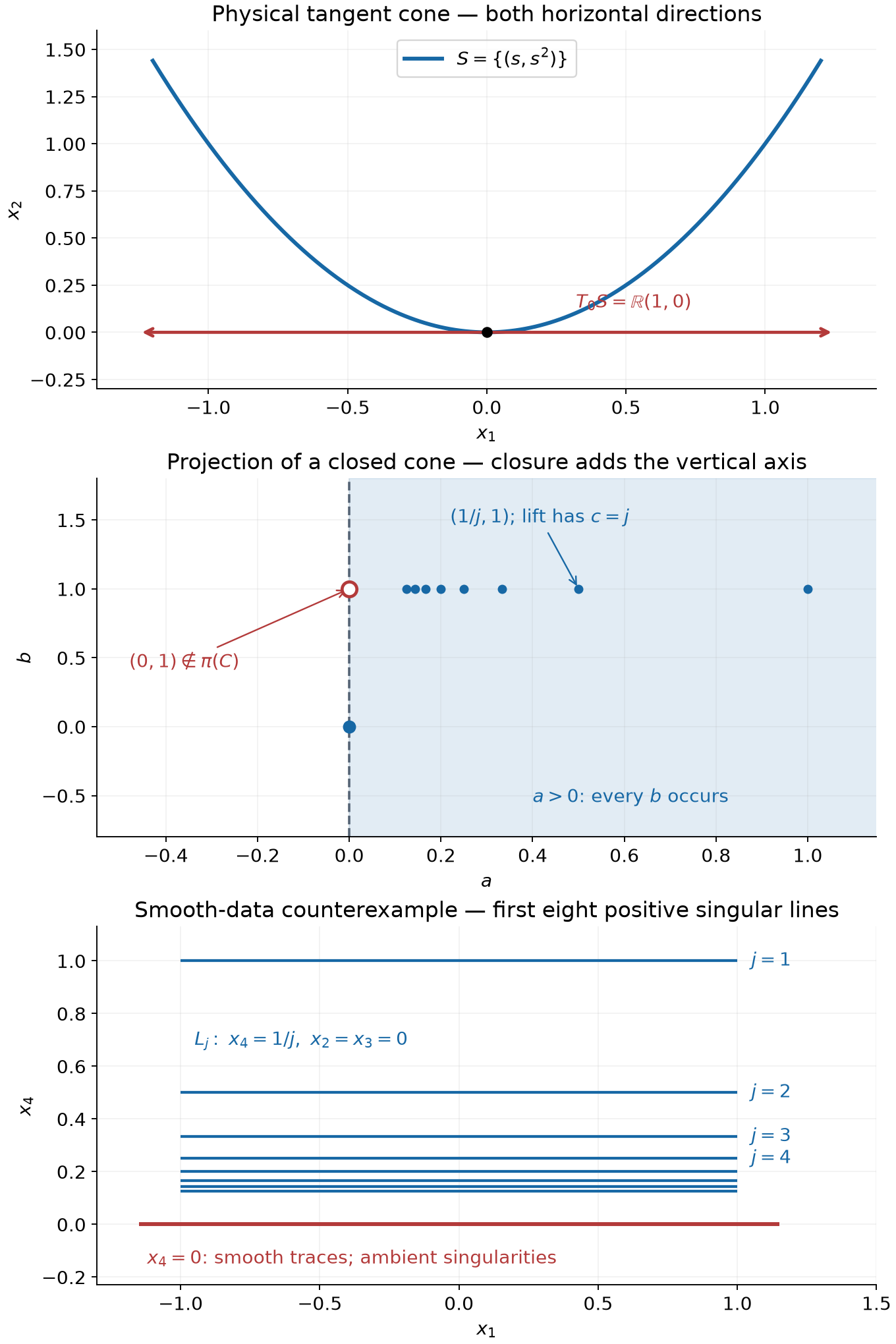
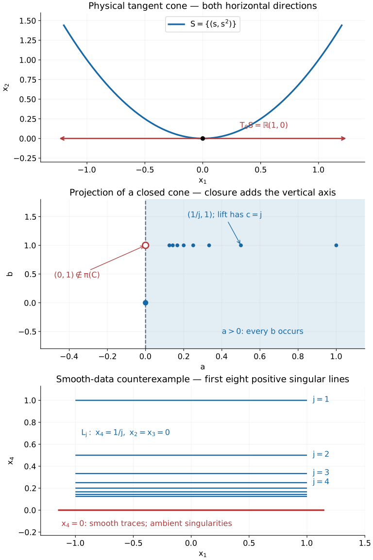
A tangent line, a nonclosed cone projection, and singular lines accumulating at a boundary

Left: the parabola has tangent cone at the origin (Exercise 2). This panel concerns physical support geometry, not a computed wavefront. Middle: projection of the closed cone onto contains and the origin, but no other point on . The indicated points tend to the missing point ; their lifts have (Exercise 3). Right: at , Proposition 10 has singular lines and their limiting line . Only the first eight positive lines are drawn. The line at zero is singular in the ambient space even though both Cauchy traces there are smooth. Vector figure · Figure source.

Exercises with complete solutions

Exercise 1 (basic) — orthant growth. Let . Compute the nearest points to and , and the profile in (T6). Compute also the profile for .

Solution. Squared Euclidean distance is the sum of independent coordinate squares. Its minimum under is attained at ; under , it is attained at . Therefore $d(\eta,-W)^2=\sum_i\max(\eta_i,0)^2,\qquad h_W(\eta)=\frac12\sum_i\min(\eta_i,0)^2. \tag{T58}$ The profile vanishes in the positive orthant and reaches in the negative orthant. This sign agrees with evaluation near for a singular covector . If , distance is , so the profile is identically zero. The strict inequality in (T7) still allows any positive rate on a compact set; it does not assert a constant uniform in .

Exercise 2 (basic) — tangent cones of a curve and its half. Compute the tangent cone at the origin of , and of . Compute in each case.

Solution. If converges and , the first coordinates are bounded, and the second coordinates tend to zero. Thus every tangent vector is horizontal. Conversely, for any real , choose , ; then . Hence . For the first coordinate is nonnegative, and the same construction with gives . Their symmetric parts are respectively the whole horizontal line and . The difference explains why both signs in (T22) impose more than membership in a one-sided tangent cone.

Exercise 3 (intermediate) — a closed tangent cone whose projection is not closed. In coordinates , let $C=\{(a,b,c):a\ge0,\ c\ge0,\ ac\ge b^2\}. \tag{T59}$ Prove that is a closed convex cone, equals its tangent cone at the origin, and has $\pi(C)=\{(a,b):a>0,\ b\in\mathbb R\}\cup\{(0,0)\}, \qquad \overline{\pi(C)}=\{(a,b):a\ge0\}, \tag{T60}$ where .

Solution. The inequalities are closed and homogeneous under nonnegative scaling. They are equivalent to $ar^2+2brs+cs^2\ge0\qquad(r,s\in\mathbb R). \tag{T61}$ For , completing the square gives . For , nonnegativity for all forces , leaving . Conversely (T61) implies by the coordinate choices; the same square computation, or the case, gives . Each inequality (T61) is a closed linear half-space in , so their intersection is convex.

If , then and , so . Conversely every rescaled point in a defining tangent sequence remains in , and closedness keeps its limit there. Thus .

For , any has a lift . For , the inequality forces . This proves the first identity in (T60); approaching through positive values proves the second. In particular , whereas the limit of its projections has no lift. The third coordinates escape to infinity, so closedness of offers no convergent lifted subsequence. This is why projection cannot in general replace its closure in Theorem 6.

Exercise 4 (intermediate) — the size and direction of the barrier. In Lemma 3 take . Determine its bound at , and explain why a small negative collar at either end suffices.

Solution. The identity , obtained directly from the exponential definitions, gives $A(1)=\frac{b}{6\cosh(\pi/b)},\qquad v(1)<-\frac{b^2}{36\cosh^2(\pi/b)}. \tag{T62}$ The quantity on the right is strictly negative for every , however small. Reflection preserves , so the majorant is unchanged and the same estimate follows from the right collar. Reflection through the origin would change the sign of and would require a different majorant. In Theorem 5 this distinction permits either missing physical normal sign to yield the same contradiction.

Exercise 5 (intermediate) — why a cylinder transfers regularity. Suppose agrees near the origin with the closed half-space . Compute and its symmetric part . If a ball in the punctured covector space misses and the cylinder avoids zero, prove that the cylinder misses .

Solution. Tangent sequences have nonnegative last coordinate. Conversely any is attained using , , which eventually lies in the given local half-space. Thus and . For every , the quantity equals . A hyperplane with such a nonzero normal therefore meets the cylinder exactly when it meets . The hypotheses of Theorem 7 hold with , ; its conclusion proves the claim. The assumption excluding zero is needed because the theorem is formulated in the punctured fiber.

Exercise 6 (intermediate) — an explicit high-frequency threshold. Suppose, on a compact real neighborhood and for , $p_m(x;\xi',\tau)=a_m(x)\tau^m+ \sum_{\ell=0}^{m-1}b_\ell(x,\xi')\tau^\ell, \qquad |a_m(x)|\ge a>0,\quad |b_\ell(x,\xi')|\le B_\ell. \tag{T63}$ Give a uniform sufficient condition for nonvanishing, allowing complex coefficients.

Solution. Put . For , the triangle inequality gives $|p_m|\ge a|\tau|^m-B|\tau|^{m-1} =|\tau|^{m-1}(a|\tau|-B). \tag{T64}$ Thus gives . If , the same conclusion follows directly. No ordering or reality of the coefficients is used. The bound controls both positive and negative normal frequencies and is uniform in the bounded tangential neighborhood, as required in Theorem 9.

Exercise 7 (advanced) — weights for accumulating singular lines. Replace in (T47) by nonzero complex coefficients satisfying $\sum_{j=1}^\infty j^N|c_j|<\infty \qquad\text{for every integer }N\ge0. \tag{T65}$ Prove that the same smooth-data counterexample and the same singular support remain valid.

Solution. The case gives absolute convergence through order two using the common compact bound for translated . Hence the sum is and solves the equation. For each specified order of tangential differentiation of either trace, (T54) bounds the -th differentiated trace by for some finite integer . Condition (T65) gives uniform absolute convergence of that derivative series on compact tangential sets. Both traces are smooth.

Near a fixed , all other translated lines are separated by a fixed positive fourth-coordinate distance. The other terms therefore have common bounds at every derivative order, by Gaussian damping. Their weighted sum is smooth by . Since , the remaining term has exactly the nonempty translated wavefront of ; no cancellation by the smooth remainder is possible. This proves (T48) with the same fixed covector and establishes singularity along every . Off the closed union, (T51) provides common derivative bounds, so the sum is smooth; closedness of singular support then includes . These are exactly the arguments proving (T55), with (T65) supplying the necessary convergence. The nonzero assumption on each is what retains each particular line.

Exercise 8 (advanced) — arbitrarily high finite regularity is insufficient. For an integer , replace in (T45) by , obtaining . Show that the translated sum with coefficients is , has smooth Cauchy data at , and still violates the smooth version of (T42).

Solution. Derivatives through order cost at most , leaving the integrable majorant on compact real sets. Thus , and the identities (T49) still prove . The integration-by-parts argument (T51), now with , proves smoothness away from : its last integrand after integrations and derivatives is bounded by , integrable for sufficiently large .

On , the -st -derivative for is $i^{k+1}A^{-1}\int_1^\infty r^{-1}e^{irx_2}\,dr. \tag{T66}$ Uniform convergence of its tails on compact positive intervals follows as in (T53), justifying the derivative. Its modulus is unbounded as , because the real part of the integral grows as and . Thus .

The translated sum converges through order . At the boundary every derivative of either Cauchy trace is bounded termwise by a polynomial in , by the same exponential estimate (T54); the weights make the derivative series converge. Near each positive line all other summands are smooth. Projection of the smooth wavefront gives a nonzero covector for at zero; the characteristic constraint (T56) excludes a pure fourth covector. Translation supplies that fixed covector at every positive line of the sum. Consequently no finite prescribed regularity, even together with smooth Cauchy data, supplies the analytic boundary conclusion.

References

Lars Hörmander, The Analysis of Linear Partial Differential Operators I: Distribution Theory and Fourier Analysis, reprint of the second edition, Springer, 2003, doi:10.1007/978-3-642-61497-2, §9.6, pp. 363–368: Gaussian scaling, tangent support, convex propagation and analytic boundary regularity. The exposition, proofs, geometric examples, integral counterexample, exercises and figure here are independently expressed. The earlier programme proofs used in the arguments are linked at their points of use.