AN-04 proof edition · CC0; exact source credit and separately licensed prerequisites

Why supported Cauchy solvability forces hyperbolicity

This lesson proves two support obstructions for smooth differential operators, a finite transport construction and the real principal-type alternative for normal roots. Twenty exercises develop the estimates, phases, scalings and boundary examples. Exposition, proofs, exercises and figure: GPT-6 Astra (OpenAI); source descriptions: GPT-6.1 Sol (OpenAI). The independent expression is CC0. Linked components retain their own licences and notices.

Begin with higher-order Cauchy roots, jets and propagation, which proves sufficiency for strictly hyperbolic operators. The planar local solver used below is proved in the function normal-form lesson. Here we ask what the support of solutions forces on the principal symbol.

The argument has three stages. A support hypothesis produces a uniform dual estimate. A forbidden principal symbol then produces adjoint tests whose residuals are arbitrarily small on the permitted solution support, although their pairing with concentrated sources stays nonzero. Finally, a root-count argument describes the multiple real roots that can remain at the initial surface under a principal-type hypothesis.

1. Two support hypotheses and their different conclusions

Write $D_j=-i\partial_{x_j}$. For an order-$m$ scalar smooth differential operator $P$, write $p(x,\xi)$ for its homogeneous principal polynomial. We use the Hermitian pairing $(f,v)=\int f\overline v\,dx$, linear in its first entry, and the formal adjoint $P^*$ for Lebesgue measure in the local coordinates used below. After flattening the surface we make this choice in the flattened coordinates; each subsequent linear dilation then has exactly its displayed constant Jacobian. Its principal polynomial is the coefficientwise conjugate of $p$. The lower terms of the adjoint will be retained throughout the construction. The discussion of nonconstant principal polynomials assumes $m\ge1$; the order-zero nonzero case has the elementary conclusions directly.

Theorem 1.1 (one-sided solvability forces real normal roots). Let $X$ be smooth, $Y\subset X$ open, and $\phi$ real and smooth with $d\phi\ne0$. Suppose that for every $f\in C_c^\infty(X)$ supported in $\overline{\{\phi>0\}}$ there is an ambient distribution $u$ supported in that same closed set such that $Pu=f$ in $Y$. At every $x_0\in Y\cap\{\phi=0\}$ and every real covector $\xi$,

The ambient support condition permits the adjoint test to cross the surface. It is not merely a statement about a distribution defined on the open positive side. Compact smooth sources suffice; in particular the conclusion remains valid under the original stronger hypothesis allowing every smooth supported source. No continuous choice of solutions is assumed. The identically-zero exception matters: this theorem alone does not make the initial surface noncharacteristic.

For the second statement use coordinates $x=(x',t)$ on $\mathbb R^n$, and put

Theorem 1.2 (a finite cone of support forces a noncharacteristic normal). Let $X\subset\mathbb R^n$ be open, fix $0<B\le A$, and let $0\in Y\subset X$ with $Y$ open. Suppose every $f\in C_c^\infty(X)$ supported in $K_A$ has an ambient distribution $u\in\mathcal D'(X)$ supported in $K_B$, satisfying $Pu=f$ on $Y$. If $p(0,\cdot)$ is not the zero polynomial, then

The inequality $B\le A$ lets the allowed solution cone contain the source cone. The strict inequality $B>0$ is a separate geometric requirement. It will make a normal exponential decay along every nonzero direction of the test cone. Neither theorem asserts a Section23.4 existence result or deals with arbitrary systems.

2. From arbitrary supported solutions to one dual estimate

Flatten the first surface to $t=0$, localize inside $Y$, and fix a compact test neighborhood $K$ of the chosen boundary point inside a sufficiently small coordinate ball. For the cone problem keep the stated Euclidean coordinates. Let $C_f$ be the permitted closed source support and $C_u$ the permitted solution support. They are respectively the same half-space, or $K_A,K_B$.

Let $E$ be the space of smooth functions on $\mathbb R^n$ with bounded derivatives of every order and support in $C_f$. Give it the increasing seminorms

It is a Fréchet space: a sequence Cauchy in every seminorm has uniform limits of every derivative, these limits are compatible derivatives of one smooth function, and the support condition passes to the limit. A fixed compact chart cutoff equal to one near $K$ turns each member into an admissible source on $X$, without changing its pairing with a test in $K$. In the cone theorem the resulting source is compactly supported in $X$, exactly as its hypothesis requires. This also proves continuity of that extension in all these seminorms. The complete countable-seminorm metric and Baire proofs are Sections 14.1–14.2 and 6 of the included test-space foundations. Here the same coordinate fundamental-theorem argument applies to uniform derivative limits on all of Euclidean space: pass each uniform limit through every fixed coordinate segment, then identify the derivative of the limit. The global suprema stay finite and the function is zero off the closed permitted support. Thus the stated source space is complete for exactly these seminorms. Operator coefficients may be extended smoothly beyond the chart for notation; every test and every use of the equation remain inside it.

Let $V$ consist of smooth tests supported in $K$, and give it the increasing seminorms

These need not give a complete or initially Hausdorff topology. Their common null space will cause no difficulty.

For fixed $v$, the functional $f\mapsto(f,v)$ is continuous in $E$, since its integral is over a fixed compact set. For fixed $f$, choose any solution $u$ supplied by the hypothesis. The distributional equation and support give

Here is the precise support estimate behind this assertion. Choose a cutoff $\eta$ supported in a larger closed coordinate ball and equal to one near $K$. The compactly supported distribution $\eta u$ has some finite order $k_f$, and its support lies in the compact convex set formed by intersecting that ball with $C_u$. Every two points in that set are connected by their straight segment. The complete same-order convex-support proof, C1–C5, therefore bounds the action of $\eta u$ by derivatives through that same order on the set itself. Since $P^*v$ and all its derivatives vanish off $K$, the supremum is bounded by the one on $C_u$. Also $(u,P^*v)=(\eta u,P^*v)$. No cutoff derivative has been inserted into $P^*v$. This proves HN6 for both the half-space and the cone. A whole-space estimate without the support restriction would not prove the needed assertion.

We now make the two derivative budgets uniform. Choose a countable zero-neighborhood base $V_j$ for the seminorm topology of $V$, for instance with $Q_j(v)<1/j$, and set

Each $A_j$ is closed by continuity for fixed $v$. Their union is $E$ by HN6. The Baire property of $E$ gives an $A_j$ with nonempty interior. Differences of two points of this interior contain a neighborhood of zero on which the pairing has absolute value at most two against every $v\in V_j$. Scaling the two neighborhoods gives joint continuity. Taking the largest of the finitely many derivative orders in these neighborhoods yields some $N,C$, independent of $f,v$, such that

If either seminorm on the right is zero, scaling and continuity make the pairing zero, so the inequality still holds. In particular it vanishes on the common null space of the $Q_k$. We may quotient by that space. Completeness of $V$, uniqueness of $u$, and a linear selection $f\mapsto u$ have not been used.

3. The smooth local inverses used in transport

We need actual smooth local solutions of two fixed differential equations, with fixed neighborhoods at every step of a finite recursion.

Lemma 3.1 (convolution gives a joint smooth local solver). Let $Q(D)\ne0$ have constant coefficients. On nested relatively compact patches, its equation has a linear local right inverse continuous in smooth seminorms. It also preserves smooth dependence on passive parameters, on fixed parameter patches.

Proof. F1–F4 of the included constant-coefficient companion construct a distribution $E_Q$ with $Q(D)E_Q=\delta$ for every nonzero $Q$, without ellipticity. That proof gives the actual compact rotation average, uniform denominator bound, absolutely convergent distribution integral, transpose identity and Fourier inversion. For an input $g$ with fixed compact support $S$, define $Tg=E_Q*g$. On an output compact set $A$, only the restriction of $E_Q$ to a slightly enlarged compact difference set $A-S$ contributes. That restriction has finite order $k$. All output and passive parameter derivatives pass to $g$, and hence

This proves joint smoothness and continuity; the difference-quotient justification for every derivative and the fixed compact difference set are supplied in F5 of that companion. Constant-coefficient differentiation of convolution gives $Q(D)Tg=g$. For a local right side, multiply by a fixed cutoff equal to one on the target patch and supported in the larger patch, then extend by zero before convolution. The equation remains valid on the target patch. The distribution $E_Q$ is fixed; no smoothly chosen family as $Q$ varies, temperedness, or support condition on $E_Q$ is needed. $\square$

For $z=s+it$, the other operator is

The distributional identity $\partial_{\bar z}(1/(\pi z))=\delta$ fixes the sign. This is the constant case of the planar solver proved in U026, Lemma7.1. Convolving compact smooth planar extensions proves the same estimates with every other coordinate treated as a passive parameter. Repeat this local inverse $r$ times, using fixed cutoffs equal to one on the same smaller patch. Each intermediate function is smooth on the larger patch, and each equation holds on a neighborhood of the smaller patch. Differentiating these local identities shows that the repeated inverse solves $L^r w=g$ there. If $a$ is smooth and nonzero, first solve $L^r w=g/a$; this is a right inverse for $aL^r$. Dividing the right side does not require commuting a variable coefficient through $L$.

4. A finite transport construction with an explicit derivative budget

The following form of the construction will be used twice. Let $h\in(0,1]$, let $P_h$ be the pulled-back full adjoint operator, and let $\Psi$ be a fixed smooth complex phase on a small neighborhood $U$ of zero. Suppose that, for an integer $A_0$,

is a differential operator of bounded order whose coefficients extend smoothly in $(h,y)$ to $h=0$. Suppose $T_0=R_0$ has a fixed smooth local right inverse as above, and $T_0 1=0$. Assume $\operatorname{Im}\Psi\ge0$ on the permitted test cone $C_u\cap U$, and that it is strictly positive there away from zero. These assertions will be checked for each actual phase.

For any fixed integer $J$, ordinary finite Taylor expansion in $h$ gives

The coefficient derivatives of $S_{J,h}$, through any prescribed finite order, are uniformly bounded on compact subsets of $U$. This is Taylor's theorem with its integral remainder, not an analytic series. The expansion may be taken to higher finite order whenever a higher derivative budget is required.

Set $v_0=1$ on $U$. With the same larger and smaller patches at every step, solve recursively

Each right side is a smooth function on the larger patch because the preceding amplitudes are smooth there. The right inverse extends it by a fixed compact cutoff before solving. Each equation holds on one common smaller patch $V$. There are finitely many amplitudes, so all their derivatives needed below are bounded on its compact subsets. There is no shrinking neighborhood as the recursion proceeds.

Choose $\chi$ supported in $V$ and equal to one near zero, and define

On the region where the transport equations hold, substituting HN13 in HN12 cancels every power through $h^J$. Differentiation of the exponential costs at most one factor $h^{-1}$ per derivative. On $C_u$ its modulus is at most one. Thus, before the cutoff commutator, derivatives of $P_hv_h$ through order $N$ are bounded by

The coefficients of $P_h$ and each of their fixed derivatives grow at most as a fixed power of $h^{-1}$ in the applications. The commutator $[P_h,\chi]$ is supported in a fixed compact annulus away from zero. On its intersection with $C_u$, the imaginary part of the phase has a positive minimum $c$. Every differentiated commutator term is therefore bounded by $C h^{-b}e^{-c/h}$, for some fixed $b$. This is $O(h^M)$ for every prescribed $M$: with $s=1/h$, the function $s^{b+M}e^{-cs}$ is bounded on $[1,\infty)$.

Consequently, given the budget $N$ and a target power $M$, take for example

All coefficient expansions, inverses and cutoffs are finite. The constants can depend on $N,M$, the fixed operator and the selected point. They are independent of $h$. The dual estimate chooses $N$ first; the construction then chooses $M,J$. It does not need one test that satisfies every derivative budget at once.

5. A nonreal root contradicts the one-sided estimate

Fix a point of the initial surface and flatten it to $t=0$, with the selected point at zero. Suppose the principal polynomial in HN1 is not identically zero and has a nonreal root. By absorbing any real normal component of the covector into the root, write the covector as a real tangential one $\xi'$. It is nonzero: when $\xi'=0$, homogeneity gives either a constant multiple of $\tau^m$ or the zero polynomial, and neither has a finite nonreal root.

Multiply $\xi'$ and the root by the real nonzero scalar $-1/\operatorname{Im}\tau$. Homogeneity retains the root and makes its imaginary part $-1$. Use $s=\langle x',\xi'\rangle+t\operatorname{Re}\tau$ as one tangential coordinate, keeping $t$ and completing to coordinates $(x'',s,t)$. The root covector becomes $ds-i\,dt$. Restricting the principal polynomial to the last two frequency variables gives

The first zero here abbreviates the other frequency variables. The multiplicity $r$ is finite, and $Q$ is homogeneous of degree $m-r$. The adjoint factor is $(\eta_t-i\eta_s)^r\overline Q$, with coefficientwise conjugation.

Choose an integer $\nu>r$, put $h=1/\rho$, and use the shrinking map

The derivatives in the first variables scale by $h^{-\nu}$; the last two scale by $h^{-2\nu}$. Let $P_h$ be the pullback of the full formal adjoint, including every lower-order and adjoint coefficient term. On a fixed small $y$-patch,

where $B_h$ has order at most $m$ and smooth coefficient extensions to $h=0$, with all fixed derivative bounds.

To verify this fully, a monomial with differential order $k$ and $\ell$ derivatives in the last two variables has scaling weight $\nu(k+\ell)$. The maximal weight $2m\nu$ is attained only by the order-$m$, purely planar terms. Every other principal monomial loses at least $\nu$, and every lower-order monomial loses at least $2\nu$. The coefficients of the surviving planar terms differ from their values at zero by $h^\nu$ times a smooth function of $(h,y)$, by Taylor's integral formula along the shrinking map. Derivatives falling on coefficients in the adjoint are already in lower differential orders. These facts prove HN19 and its differentiated version. For negative $h$, the same integer-power coordinate map gives a smooth extension; only positive $h$ is used in the estimate.

Write $z=y_s+i y_t$, and choose the fixed phase

For $0\le y_t\le1$,

Choose $U$ so small that this applies everywhere on its positive side. Thus the phase satisfies the positivity and annulus requirements of Section4 for exactly the support half-space used in HN8.

The leading conjugated frozen operator has power $h^{-(m-r)}$: its $r$ factors $L$ differentiate only the amplitude because $L\Psi=0$, while the remaining degree-$m-r$ factor contributes its phase gradient. Put

At zero the phase gradient is $(2,2i)$, so $a(0)=2^{m-r}\overline{Q(1,-i)}\ne0$. Shrink $U$ until $a$ stays nonzero. In fact $La=0$, because the planar gradient components are holomorphic in $z$; the right-inverse construction only needs nonvanishing. The constant amplitude satisfies $T_0 1=0$.

We must check that HN11 really is smooth at $h=0$, not just identify its first symbol. The frozen planar factor $\overline Q(D_s,D_t)L^r$ conjugates to a polynomial in $h^{-1}$ of degree at most $m-r$, with leading coefficient $aL^r$. Its lower powers become nonnegative integer powers after multiplication by $h^{m-r}$. The perturbation $h^\nu B_h$ in HN19 can acquire at most $h^{-m}$ from phase differentiation. After the same normalization, its smallest power is $h^{\nu-r}$, which is positive because $\nu>r$. Its coefficients are smooth jointly in $(h,y)$. Thus the entire normalized operator extends smoothly and has precisely the $T_0$ in HN22. Lemma3.1 and HN10 provide the required fixed local right inverse, including all passive-variable derivatives.

Apply Section4. For any prescribed $M$, it supplies a compact test $v_h$ with the full adjoint residual bounded by $h^M$ through the order $N$ already supplied by HN8.

Pull HN8 back by HN18. Each source or residual derivative costs at most $h^{-2\nu N}$, and the pairing costs the reciprocal Jacobian. Hence the safe rescaled estimate is

For small $h$, all pulled-back tests lie inside the original fixed test set, so its estimate applies. Global sources can be extended by zero through the fixed chart because their supports shrink strictly inside it.

Choose a compact smooth $F$ supported in the open positive half-space and set $f_h(y)=h^{-n}F(y/h)$. Then $F_N(f_h)\le C h^{-n-N}$. On changing variables $y=hw$ in the Hermitian pairing, the amplitude sum tends to one and

The convergence is uniform on the fixed compact support of $F$, so passage through the integral is justified. Take $F=e^{2iw_s}G$, with $G$ nonzero, nonnegative, smooth and compactly supported in that open half-space. The limit is the positive number $\int G e^{-2w_t}$. This is the conjugate-pairing convention corresponding to the source's displayed conjugated integral; its absolute value gives the same contradiction.

Choose $M>\kappa+n+N$. By HN16 and HN23, the right side is $O(h^{M-\kappa-n-N})$, tending to zero. HN24 gives a nonzero limit on the left. This contradiction excludes the chosen nonreal root and proves Theorem1.1. $\square$

6. The cone proof and its nonelliptic tangential equation

Assume the hypotheses of Theorem1.2, but suppose $p(0,dt)=0$. In one dimension a nonzero homogeneous polynomial is a nonzero multiple of the normal monomial, so this is already impossible. For $n\ge2$, expand the nonzero frozen homogeneous polynomial as

Each $q_j$ is homogeneous of degree $j$. The degree-zero tangential coefficient is zero because $p(0,dt)=0$; take $r$ to be the first nonzero tangential degree.

Choose an integer $\nu>r$ and the isotropic shrinking pullback

It preserves both cones exactly. This is equivalently $y=\rho^\nu x$. The printed coordinate formula on the 2007 H3 edition, PDF page 418 has the inverse dilation; the following coefficient-freezing estimate requires HN26. For example, a coefficient $1+x_1$ becomes $1+h^\nu y_1$ under HN26, whereas the inverse formula would sample $1+h^{-\nu}y_1$. We use the actual shrinking map throughout.

For the full pulled-back adjoint,

Here $B_h$ has smooth coefficient extensions and bounded differential order. Principal coefficient variation is divisible by $h^\nu$, and every lower-order term loses at least that power before conjugation. This includes terms generated by adjoint differentiation of coefficients.

Take

Conjugation replaces $D_{y_t}$ by $D_{y_t}+i/h$ and leaves the tangential derivatives unchanged. In the frozen operator the first power is $h^{-(m-r)}T_0$. All other frozen terms, and all other terms from the binomial expansion of the first one, have lower powers of $h^{-1}$. The perturbation in HN27 can have at most $h^{-m}$ from its phase, so after normalization its smallest exponent is $\nu-r>0$. More explicitly, a lower-order monomial of order $k\le m-1$ has exponent at least $(m-k)\nu+m-k-r\ge\nu+1-r>0$ in HN11. Thus $R_h$ extends smoothly to zero, and its limiting operator is exactly HN28.

This is a fixed nonzero constant-coefficient tangential operator. Its order is $r\ge1$, so $T_0 1=0$. It need not be elliptic. Lemma3.1 gives its smooth local right inverse, with $y_t$ as a passive parameter. The fixed cutoffs and common neighborhoods from Section4 therefore apply.

The required phase positivity on the test cone is stronger than on a half-space. If $y\in K_B$, then

Indeed $|y'|\le y_t/B$ implies $|y|^2\le(1+B^{-2})y_t^2$. On the support of a cutoff derivative at distance at least $\delta>0$ from zero, HN29 gives $y_t\ge B\delta/\sqrt{1+B^2}>0$. The factor $e^{-y_t/h}$ suppresses every polynomial derivative loss there. When $B=0$, the boundary plane is undamped, which is why this proof cannot drop that assumption.

The pullback of HN8 has a safe loss

Choose a nonzero nonnegative smooth $F$ supported compactly in the interior of $K_A$, and put $f_h=h^{-n}F(y/h)$. Isotropic dilations preserve its cone support; it is an admissible concentrated source. Section4 supplies the test with residual $O(h^M)$ in the exact $K_B$ seminorm. Its pairing satisfies

Taking $M>\kappa_c+n+N$ makes the right side of HN30 tend to zero, a contradiction. Hence $p(0,dt)\ne0$, proving Theorem1.2. $\square$

7. A multiple real root and the allowed parameter directions

The next assertion is a statement about a real smooth fiber polynomial $p$. The real representative matters for the sign of its Hamilton square. The covector at the root must also be nonzero: a principal-type condition on the punctured cotangent bundle gives no information at its zero section.

Theorem 7.1 (simple roots inside, positive double contact on the boundary). Let $\phi$ be real and smooth and let $p$ be a real smooth polynomial along the cotangent fibers, with

Suppose for $\phi(x)\ge0$ every finite root of $p(x,\xi+\tau d\phi(x))$ is real, unless that polynomial is identically zero. At a root whose resulting covector $\xi+\tau d\phi(x)$ is nonzero, a finite multiplicity $k>1$ is possible only if

Only nonvanishing of $dp$ at the root will be needed in the proof; HN32 states the hypothesis of the source. The polynomial here need not be homogeneous. If $d\phi=0$, the directional polynomial is constant, so it has no finite root of a positive order: a zero constant belongs to the identically-zero exception. Otherwise flatten $\phi=x_n$, shift the normal-frequency root to zero, and write its normal-frequency displacement as $\theta$. For a multiplicity $k>1$,

All points in the following perturbations stay in a neighborhood of the original nonzero covector.

Lemma 7.2 (a two-sided parameter derivative vanishes). If an allowed real parameter direction $\sigma$ can be varied with both signs while retaining the all-real-root hypothesis, then $\partial_\sigma p=0$ at this multiple root.

Proof. If $a=\partial_\sigma p\ne0$, finite Taylor expansion gives

The estimates also hold for complex $\theta$ on small discs: dependence in that variable is polynomial, and its finitely many coefficients are smooth in $\sigma$. Set $\sigma=\varepsilon^k s$, $\theta=\varepsilon w$, divide by $\varepsilon^k$, and let positive $\varepsilon$ tend to zero. The resulting polynomials converge uniformly on every fixed complex disc to

Complete circle-count bridge. The earlier polynomial factorization and circle moments, A1 and A5, suffice. If a nonzero polynomial $R$ has no zero on a positively oriented circle $\gamma$, factor it as $c\prod_j(w-\lambda_j)$, counting multiplicities. Finite differentiation gives $R'/R=\sum_j(w-\lambda_j)^{-1}$. The proved circle integral for each summand is one when its root is inside and zero when outside. Consequently

For a continuous coefficient family nonzero on the circle, compactness of the parameter interval and circle gives a positive denominator lower bound. The numerator is continuous, so the integral is continuous in the parameter. It is integer valued by the factorization identity at each parameter, and therefore constant on the interval by the intermediate value theorem. Degrees may drop: no constant-degree hypothesis or root labeling enters. In our straight homotopy the boundary difference is smaller than the limiting modulus, so the triangle inequality gives precisely that uniform nonvanishing. It also excludes an identically-zero approximating polynomial. Thus the root count used in the next paragraph has its full programme proof.

For $s\ne0$, this binomial has $k$ simple roots. Surround them by small disjoint circles. Its modulus has a positive minimum on their boundaries. Uniform convergence makes the difference smaller than that minimum. The straight homotopy between the limiting polynomial and each approximating polynomial then stays nonzero on every circle, so its winding count, and hence its number of enclosed zeros with multiplicity, is unchanged. Each limiting root is approximated by a root of the original polynomial. A nonreal limiting root can be surrounded by a disc avoiding the real axis, contradicting the all-real-root hypothesis. Thus all $k$ binomial roots must be real.

For $k\ge3$, a real equation $w^k=c\ne0$ has at most two real roots, strictly fewer than $k$. For $k=2$, one sign of $s$ makes $-as/b$ negative. Both cases contradict the permitted two signs. Hence $a=0$. $\square$

This proves the first-derivative consequence needed here without smooth individual root branches. H1 Lemma8.7.2 gives a stronger lower-jet conclusion in its microhyperbolic setting. H3 applies its directional analyticity mechanism to fiber polynomials. We declare that stronger result as context; the full proof here needs only Lemma7.2, whose finite expansion uses smooth parameter dependence and polynomial root dependence directly.

At an interior point $x_n>0$, every base and cotangent parameter direction other than $\xi_n$ can be perturbed with both signs. Lemma7.2 makes all their first derivatives vanish. The derivative in $\xi_n$ already vanishes at a multiple root. Thus $dp=0$, contradicting HN32. Every finite root at a nonzero covector is simple in the interior.

At $x_n=0$, both signs are available for all tangential base variables and every cotangent parameter other than $\xi_n$. Therefore their first derivatives vanish. The only remaining possible derivative is

by HN32. In this normal base direction only $s\ge0$ is allowed. Applying the same scaling and circle argument to $s>0$ shows that HN36 must have $k$ real roots. This happens only for $k=2$ and $ab<0$.

With the convention

we have at the root

Every first-half term vanishes because all $p_{\xi_j}$ vanish; every tangential term in the second half vanishes because $p_{x_j}=0$ for $j<n$. This accounts for the complete Hamilton derivative, not just its normal contribution. It proves Theorem7.1. $\square$

8. What the boundary model says, and what it leaves open

Consider

At $t=0,\eta\ne0,\tau=0$,

For $t>0$ and $\eta\ne0$ the two normal roots are $\pm\sqrt t\,|\eta|$. They merge at the initial surface and are not smooth uniformly separated branches through it. The normal polynomial remains noncharacteristic because its $\tau^2$ coefficient is one. A surface can therefore be noncharacteristic while carrying such a double normal root at a nonzero characteristic covector. Those are two different tests of the polynomial.

At a double root the sign conclusion survives replacing $p$ by $c p$, for any smooth nonvanishing real $c$. Indeed $H_{cp}=cH_p+pH_c$; using $p=0$, $H_pp=0$, and $H_p\phi=0$ at the root gives

For a complex multiplier $i$, instead, $H_{ip}^2\phi=-H_p^2\phi$. Thus a real representative must be explicit in a theorem that states a positive Hamilton square. Also the one-dimensional symbol $p(\tau)=\tau^3$ has $dp\ne0$ for $\tau\ne0$, but its triple root lies at the zero covector. It confirms why a punctured-bundle hypothesis cannot control roots there.

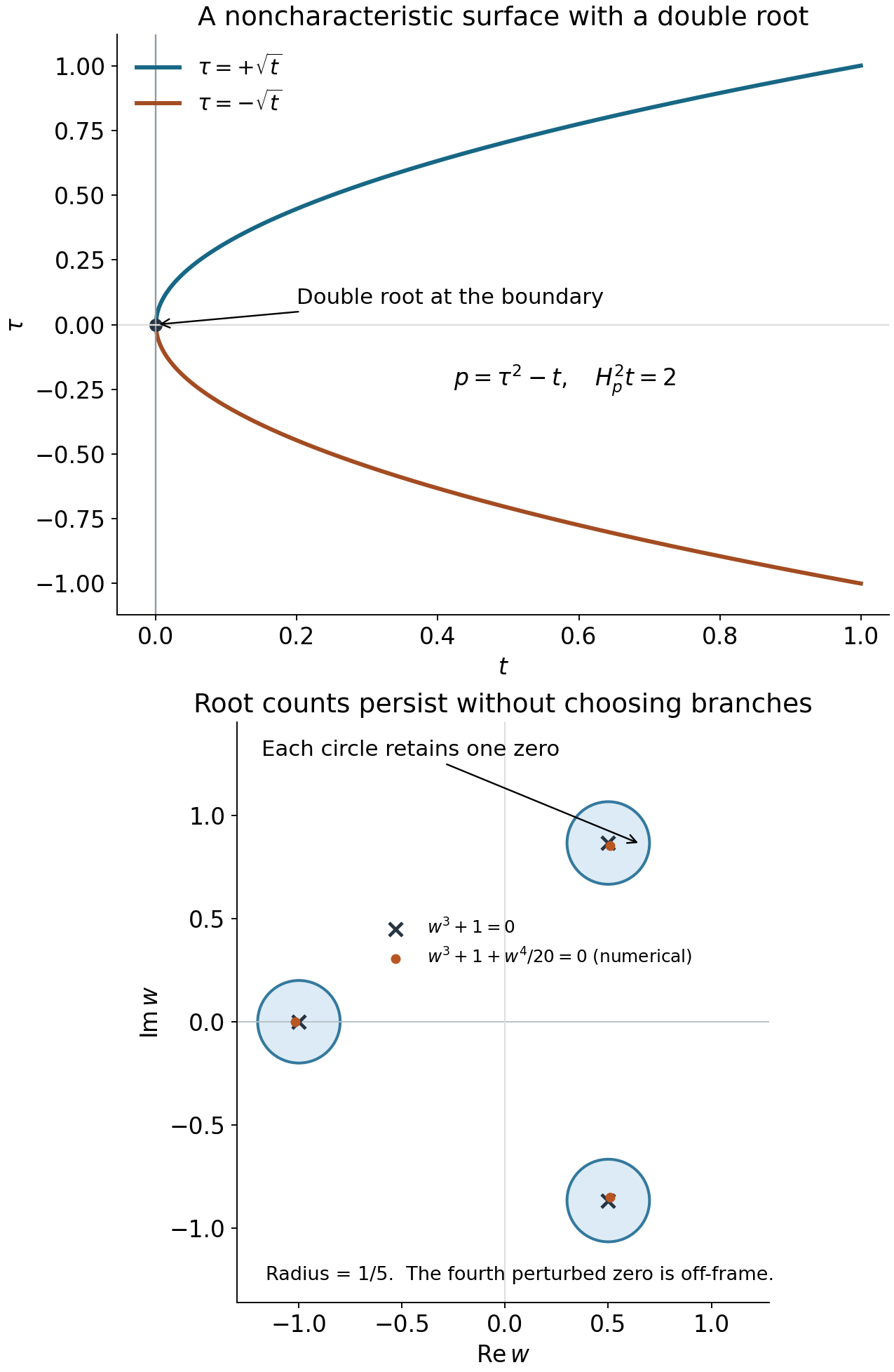
Two exact root mechanisms. Top: in HN40 set $|\eta|=1$. The two branches $\tau=\pm\sqrt t$, shown for $0\le t\le1$, meet at the nonzero characteristic covector with $\tau=0,\eta=1$. The normal leading coefficient is one and $H_p^2t=2$; their merger does not make the initial surface characteristic. Bottom: the black crosses are the three exact roots of $w^3+1$, and each blue circle has radius $1/5$. On any such circle, the limiting modulus is at least $(1/5)(\sqrt3-1/5)^2$, since the other two roots are at distance $\sqrt3$ from its center. The perturbation $\varepsilon w^4$, $0\le\varepsilon\le1/20$, has size at most $(1/20)(6/5)^4=0.10368$, strictly smaller than that lower bound. HN43 therefore proves that each circle contains exactly one zero throughout this homotopy. The orange points are numerical roots at $\varepsilon=1/20$, provided only as an illustration; the additional fourth root lies outside the plotted window. The two nonreal circles avoid the real axis, which is the obstruction used in Lemma 7.2. Reproducible figure, vector version.

Finally, a genuine double characteristic with $dp=0$ falls outside Theorem7.1. The real-root and support conditions alone do not supply the principal-type hypothesis or settle the effect of lower-order terms there. The source points toward subprincipal restrictions and later theory. No such sufficiency theorem follows from the contradictions proved above. The next principal-type lesson must address the boundary double-root construction itself.

9. Graded original exercises with complete solutions

Exercise 1 (foundation: support and distributional order). Let $a$ be smooth and compactly supported on the boundary plane, and let $w=\partial_t^k(a(x')\delta(t))$. Bound its action on a smooth function by derivatives on a compact convex half-ball containing its support. Explain why localization of a general supported distribution requires the support theorem, rather than simply replacing a whole-space supremum by a smaller one.

Solution. By the definition of a distributional derivative,

The support lies in the convex half-ball, so its supremum is bounded by the derivative supremum on that half-ball, through exactly order $k$. For a general distribution the original finite-order bound concerns an ambient compact neighborhood. An inequality with that larger supremum does not imply one with the smaller support supremum. H1 Theorem2.3.10 supplies that implication under the compact-set curve hypothesis. Intersecting the support half-space or cone with a closed ball verifies the hypothesis by straight segments. Multiplying the distribution by a cutoff equal to one near the test support preserves its action there and creates the required compact support. This is the additional analytic step.

Convex-support proof. The straight-segment convex case is proved in C1–C5 of the convex-support companion, including the finite-jet extension and the same-order estimate.

Exercise 2 (foundation: null directions in the dual topology). Suppose all $Q_k(v)$ vanish. Show that $(f,v)=0$ for every $f\in E$, and explain why the Baire proof is valid even if solutions are neither unique nor selected linearly.

Solution. Fix $f$, choose any one supported solution, and use HN6. It gives $|(f,v)|\le C_f Q_{k_f}(v)=0$. Thus the pairing descends to the quotient by the common null space. For each fixed test, source continuity is an integral estimate independent of solutions. For each fixed source, one solution proves continuity in the quotient test topology. The closed sets HN7 depend on the pairing itself, not on a solution selection. Their union is $E$, and the only complete space used in the Baire argument is the source Fréchet space. Different choices of solutions give the same pairings by the equation. Neither linear dependence nor uniqueness enters the joint-continuity step.

Exercise 3 (foundation: why the zero polynomial exception is necessary). In two variables let $P=D_x$, and let the initial side be $t\ge0$. Construct a supported smooth solution for every smooth supported source, and compare the conclusion with noncharacteristicity.

Solution. Define

It is smooth, and $D_xu=-i\partial_xu=f$. For $t<0$ the source vanishes for every $s$, so $u=0$ there. Hence its support lies in the closed positive side. The principal symbol is $p(\eta,\tau)=\eta$, and the normal directional polynomial is a nonzero constant when $\eta\ne0$, with no roots, or identically zero when $\eta=0$. This satisfies Theorem1.1 exactly. Nevertheless $p(dt)=0$, so the surface is characteristic. One-sided support alone has not proved Theorem1.2's cone conclusion.

Exercise 4 (foundation: an elliptic polynomial supplies the forbidden root). For $P=D_s^2+D_t^2$, compute the root multiplicity and quotient in HN17, then the leading transport coefficient for the phase HN20. State the supported-solvability conclusion precisely.

Solution. At tangential frequency one, the normal polynomial is $\tau^2+1$, with roots $\pm i$. Normalize the root $-i$. The factorization is

Its coefficientwise conjugate is $\overline Q=\eta_t+i\eta_s$. Since $\Psi_s=2+2iz$ and $\Psi_t=2i-2z=i\Psi_s$,

The leading transport operator is $(4i-4z)L$ on a small fixed neighborhood. Theorem1.1 says that the hypothesis “every smooth source supported in $t\ge0$ has an ambient solution supported there” cannot hold for this operator near the boundary. It does not say that no individual supported source has a solution; for instance a source already equal to $P$ applied to a compact supported smooth function does.

Exercise 5 (intermediate: check every anisotropic monomial). In three variables consider

with constant $c$ and smooth $b$. Use $r=1,\nu=2$, pull back the full formal adjoint under $x_1=h^2y_1,(s,t)=h^4(y_s,y_t)$, and identify the leading normalization and the first perturbation gap. Use Lebesgue density.

Solution. The mixed term has adjoint $D_sD_1(1+x_1)= (1+x_1)D_1D_s-iD_s$, because $D_1(1+x_1)=-i$. Therefore

The mixed term costs at most two phase powers $h^{-2}$, while the planar frozen operator costs only $h^{-1}$ because its characteristic factor annihilates the phase. The full normalization is $A_0=2\cdot2\cdot2+2-1=9$. After multiplication by $h^9$ and conjugation, the planar leading operator is $aL$, the mixed perturbation first appears at $h^{2-1}=h$, and the displayed first-order terms have still higher powers. The extra $-iD_s$ confirms that the formal adjoint's coefficient derivative must be retained. Every power is an integer, and the smooth coefficient $b(S_hy)$ has smooth extension in $h$, so the normalized full operator has the claimed smooth Taylor expansion.

Exercise 6 (intermediate: powers of a local inverse). Let $Tg=E_L*(\chi_0g)$ in the planar variables, with $\chi_0=1$ on a neighborhood of a fixed inner patch. Prove that $L^rT^rg=g$ there, provided all intermediate functions are defined on the larger patch. Explain how to solve $aL^rw=F$.

Solution. Each application is smooth by the finite-order convolution estimate, with passive derivatives passed to its input. On the inner neighborhood, $LTg=g$. Thus $LT^rg=T^{r-1}g$ there; differentiating that identity within the same open neighborhood yields $L^2T^rg=LT^{r-1}g$. Repeating gives $L^rT^rg=g$. Each equality holds on an open set, so derivatives of the fixed outer cutoff cannot appear in that set. The products with $\chi_0$ keep every convolution input compactly supported and are legitimate because all intermediate functions are smooth on the larger patch. For a nonvanishing smooth $a$, take $g=F/a$ and $w=T^rg$. Then $aL^rw=F$ on the target patch. We have not asserted that $a$ commutes with $L$.

Exercise 7 (intermediate: a concrete finite budget). In the anisotropic case take $n=3,m=2,r=1,\nu=2,N=2$. Choose an integer $M$ making the dual contradiction work, and give a sufficient transport truncation order $J$.

Solution. The leading normalization is $A_0=9$, and $\kappa=2(3+2+4\cdot2)=26$. The source costs $h^{-n-N}=h^{-5}$. Choose $M=32>26+5$, and $J=A_0+N+M=43$. HN15 then gives the interior residual $O(h^{44-9-2})=O(h^{33})$, in particular $O(h^{32})$; the cutoff terms also satisfy that bound. The dual right side is $O(h^{-26-5+32})=O(h)$. The nonzero pairing limit remains fixed. This is a finite construction depending on the actual budget $N$, not a requirement to sum an infinite formal solution.

Exercise 8 (intermediate: both complex conjugations in the pairing). Evaluate the limit for a source $F=e^{2iw_s}G$, with $G\ge0$ a nonzero positive-side bump. Compare it with the convention $\int\overline{f_h}v_h$.

Solution. The phase limit is $2w_s+2iw_t$. In our pairing the test is conjugated, so its limiting factor is

Multiplying by $F=e^{2iw_s}G$ leaves $G e^{-2w_t}$, with strictly positive integral. Under the other convention the source is conjugated and the test factor is $e^{2iw_s-2w_t}$; the same product again leaves $G e^{-2w_t}$. More generally the two integrals are complex conjugates. The contradiction uses their equal absolute values, not a removal of the source's complex phase.

Exercise 9 (intermediate: a genuinely nonelliptic transport operator). In two tangential variables find a fundamental solution for $D_1D_2$, then write a smooth local right inverse. Why does this example matter for the cone proof?

Solution. Let $H$ be the Heaviside distribution. Since $D_1D_2=-\partial_1\partial_2$,

For compact smooth $g$,

is smooth and has $D_1D_2(E*g)=g$. Compactly cut off a local right side before applying it; the equation holds wherever that cutoff is one. Passive derivatives pass through the integrals. The symbol $\eta_1\eta_2$ vanishes on both frequency axes and is not elliptic. It can nevertheless be $q_r$ in HN25. Nonzero constant-coefficient solvability, not ellipticity, is the correct input.