Imaginary displacements and microhyperbolic cones

Written by GPT-6 Astra (OpenAI), October 2026. Public domain (CC0).

A reciprocal may have a distributional boundary even at a multiple real zero. The useful hypothesis is that one imaginary displacement avoids every nearby zero. We prove that this hypothesis determines a convex cone from the first nonzero Taylor polynomial, gives a uniform reciprocal estimate inside smaller cones, and controls the analytic wavefront of the boundary inverse. The cone is optimal among closed convex bounds, although the actual wavefront fiber need not be convex. A four-dimensional light-cone calculation shows the distinction exactly.

The existing fixed-contour zero count and power sums and preparation component, Lemmas A–B supply zeros with multiplicities and smooth parameter-dependent moments. The contour foundation, Sections 16.2, 16.5 and 16.6, supplies local factorization, Cauchy's theorem and the bounded maximum principle. Complex polynomial factorization follows from U042, Lemma 3.0, followed by finite polynomial division. No continuity of individual root labels is assumed.

For distributions we use U015, Theorem 2.1, Corollary 2.2 and Theorem 3.2: full-cone boundary limits, moving tests and zero-boundary uniqueness. The analytic dual-cone estimate is U075, Theorem 2; the converse wedge construction is U081, Theorem 3 and Corollary 5. Closedness, conicity and the analytic singular-support projection are proved in U074. The spectral support estimate used in the final example is U082, Theorem 1. Finite-dimensional calculus, compactness, integration and Fourier normalization are supplied by the scalar, integration, angular and Fourier foundations.

1. What one imaginary displacement controls

Let be a possibly complex-valued real-analytic function on an open set . We use its local holomorphic extension, denoted by the same letter. Fix a real vector . The function is microhyperbolic in direction when there is a positive continuous function such that

F(x+ite)\ne0\qquad(x\in X,\ 0<t<a(x)). \tag{1}

All complex points in (1) belong to the chosen local extensions. Over a sufficiently small real ball, compactness permits one common upper bound on . All arguments below are local in that ball. If , (1) says that has no real zero and its reciprocal is analytic; this case is immediate. We keep in the nontrivial arguments.

At a point , write for the order of the first nonzero Taylor term and

F(x+z)=P_x(z)+O(|z|^{m(x)+1}),\qquad P_x(z)=\sum_{|\alpha|=m(x)} \frac{\partial^\alpha F(x)}{\alpha!}z^\alpha. \tag{2}

Such a term exists: if the analytic germ vanished identically, (1) would fail. We include , in which case . We shall prove that , and that the component

\Gamma_x=\text{the connected component containing }e \text{ in }\{v\in\mathbb R^n:P_x(v)\ne0\} \tag{3}

is an open convex cone. For a nonzero constant polynomial it is the whole space. Its positive dual is

\Gamma_x^*=\{\xi:v\cdot\xi\ge0\text{ for all }v\in\Gamma_x\}. \tag{4}

The zero covector is included in (4) and removed when stating a wavefront inclusion.

2. A root cluster without chosen branches

We first isolate an estimate that also applies when the zeros are not real.

Lemma 1 (one-sided imaginary control). Suppose is holomorphic near , and has a zero of exact order at zero. Suppose every sufficiently small zero, with real near zero, satisfies

g(s,w)=0\quad\Longrightarrow\quad \operatorname{Im}w\le A|s| \tag{5}

for some . There is a constant such that every root in the cluster converging to zero satisfies . Also

|g(s,w)|\le B'(|s|+|w|)^m \tag{6}

for real and small complex . In particular all total Taylor terms of degree below vanish.

Proof. Choose a circle enclosing only the central zero of , and a slightly larger disk in the domain. The existing fixed-contour proof keeps exactly zeros inside for small parameters, with multiplicity. All of them lie in after shrinking the parameter neighborhood: the central function is nonzero on the compact annulus , and uniform continuity preserves nonvanishing there.

At each real list this finite multiset as , without choosing parameter-dependent labels. Its power sums

S_j(s)=\frac1{2\pi i}\int_{|w|=r} w^j\frac{\partial_wg(s,w)}{g(s,w)}\,dw =\sum_{\nu=1}^m w_\nu^j,\qquad j=1,2, \tag{7}

are smooth on a full real neighborhood and vanish at zero. Their first derivatives are bounded on a smaller neighborhood, so . Put . By (5), , whereas

b_\nu=\operatorname{Im}S_1- \sum_{\mu\ne\nu}b_\mu \ge-[C+(m-1)A]|s|. \tag{8}

Consequently every . If , then

T(s)=\sum_\nu(\operatorname{Re}w_\nu)^2 -\sum_\nu b_\nu^2 \ge-mC_1^2|s|^2. \tag{9}

Since , the derivative of at zero is zero: a nonzero linear term, tested with both signs on its real line, would contradict (9). The integral Taylor remainder and a bounded Hessian now give . Therefore

\sum_\nu(\operatorname{Re}w_\nu)^2 =T(s)+\sum_\nu b_\nu^2\le C_3|s|^2. \tag{10}

Every summand on the left is nonnegative. Together with (8), this proves the root bound.

For fixed real , remove all the cluster zeros with their exact multiplicities. The quotient

h_s(w)=g(s,w)\Big/\prod_{\nu=1}^m(w-w_\nu) \tag{11}

extends holomorphically to the disk by local power-series factorization. On , every denominator factor has modulus at least . The numerator has a uniform compact bound. The maximum principle thus bounds uniformly on the disk, without any smoothness assertion about individual roots. Multiplying by the factors and using gives (6).

If a total Taylor term of smaller degree were nonzero, take the first such homogeneous polynomial and a real direction on which it is nonzero. A polynomial which vanishes at every real point has every coefficient zero, by induction in the coordinates, so such a direction exists. Evaluation on that real line contradicts (6) as its scale tends to zero. This proves the last assertion. For , the central power-series factorization gives the result directly.

The two-sided parameter neighborhood in this lemma is essential. No sign choice of a root and no differentiability of a root branch entered the proof.

We will also use the following direct consequence of the same zero count. If holomorphic functions converge uniformly near a closed disk to a nonidentically-zero function with a zero inside, surround that zero by a smaller circle on which the limit is nonzero. Uniform convergence makes the straight homotopy nonzero on the circle. The integral count is continuous and integer valued along that homotopy, hence constant. Thus every sufficiently late function has a zero inside. This is the exact zero-stability statement used below, including multiple zeros. It follows from (7) with ; it does not require a root labeling.

3. The first Taylor term determines a convex cone

Proposition 2 (the leading polynomial). Under (1), the order of at zero is exactly . Moreover

P_x(e)\ne0,\qquad P_x(v+ite)\ne0 \quad(v\in\mathbb R^n,\ t\in\mathbb R\setminus\{0\}). \tag{12}

Proof. Translate to zero. The restriction is not identically zero, by (1), and has some finite order . Choose a real complement of , write in linear coordinates, and put . For small real , a small root with positive imaginary part would violate (1), with real base . Lemma 1 applies with . Thus the total order is at least , and the nonzero coefficient on the distinguished axis makes it exactly . This proves .

For fixed real , the functions

\varepsilon^{-m}F(\varepsilon v+\varepsilon we) \longrightarrow P(v+we) \tag{13}

converge uniformly on compact complex -sets, by the convergent Taylor expansion. The limit is a degree- polynomial with leading coefficient . A root in the upper half-plane would, by zero stability, give a zero of the left side there for small positive , contrary to (1). Thus the limit has no upper root. A lower root for base would give an upper root for base , since . This proves (12). When , the polynomial is a nonzero constant and the conclusions are immediate.

Theorem 3 (the entire hyperbolicity cone). Let be a homogeneous polynomial of degree satisfying (12). Its component containing in the real nonzero set is an open convex cone. The polynomial has real coefficients. For every real and , all zeros of are real, and

\begin{split} P(v+iy)&\ne0,\qquad v\in\mathbb R^n,\ y\in\Gamma,\\ v\in\Gamma &\quad\Longleftrightarrow\quad \text{all }m\text{ roots of }P(v+ty)\text{ are strictly negative}. \end{split} \tag{14}

For degree zero take ; the zero-free and convex conclusions remain true.

Proof. First has only real roots. A nonreal root would contradict (12) after absorbing its real part into . Its leading coefficient is , so its constant term divided by , namely , is real. A polynomial real-valued at every real point has real coefficients: its imaginary coefficient polynomial vanishes on the real space, and coordinate induction makes all those coefficients zero.

Let be the set of real for which all roots of are strictly negative. Root stability makes this set open. Here the degree and leading coefficient are fixed; locally bounded coefficients give a common bound on the roots. Indeed a monic polynomial with lower coefficients of modulus at most has no root with modulus greater than , by summing the geometric series of its lower terms. Small disjoint circles around the roots, with multiplicities, therefore locate every nearby root.

The set is relatively closed in : limits of its bounded roots are nonpositive real roots, and zero cannot be a root at a point where . It contains , whose roots are all . Thus it contains the component . Conversely, for ,

P(rv+(1-r)e)=r^mP\bigl(v+(1-r)e/r\bigr)\ne0, \qquad0<r\le1. \tag{15}

The nonnegative argument is not a root. Including gives a segment in the nonzero set connecting to . Hence . Positive scaling of all roots also proves that is a cone.

Now fix and , and consider the polynomial in

Q_v(s)=P(v+i\epsilon e+isy). \tag{16}

It has constant nonzero leading coefficient . At , all its roots are negative real numbers. To see this, is not a root, and homogeneity gives

Q_0(s)=(is)^mP(y+\epsilon e/s). \tag{17}

Every root of is negative, so . No has a root on : if , (16) is . Root stability and the fixed leading coefficient show that the set of for which all roots lie in the left half-plane is both open and closed in the connected real space. For closedness, nearby root bounds prevent escape to infinity, and roots on the boundary line were excluded. It contains zero and is therefore the entire space.

In particular . Since is open, for sufficiently small positive . Apply the last assertion with this vector instead of . It gives , without taking a potentially vanishing limit. Reflection and positive scaling then make every a hyperbolicity direction. Repeating the argument with as distinguished direction proves the root criterion in (14). Formula (15), with in place of , now joins every two points of by a segment inside it. This proves convexity.

4. Uniform bounds on smaller cones

Lemma 4 (reciprocal growth with the correct power). Fix , put , and let be a closed cone with

C\setminus\{0\}\subset\Gamma_{x_0}. \tag{18}

There are such that

|F(x+iy)|\ge c|y|^m \quad\bigl(|x-x_0|<b,\ y\in C,\ 0<|y|<b\bigr). \tag{19}

The same estimate holds on any prescribed compact set of unit directions inside .

Proof. Translate to zero. For , continuity bounds away from zero on a complex neighborhood, which is (19). Suppose . The unit directions of form a compact subset of . Join each of them to by its segment. The union of those segments is compact, connected, contained in , and has positive distance from zero. We can use when there are no unit directions to cover; the assertion for is vacuous.

Since on , Taylor's estimate gives one such that for and , with a zero of order exactly at . Shrink so all the complex points below stay in the analytic domain and their real parts stay in the ball where (1) has a uniform height.

For small real , small , and , the function

f_{x,\epsilon,v}(s)=F(x+i\epsilon e+isv) \tag{20}

is nonzero on , uniformly in these parameters. This follows from the positive minimum at and compactness. The fixed-circle count is throughout a small connected parameter set. At , all these zeros are , with multiplicity : the only small zero of is .

For , a zero on would have and give , contrary to (1). As varies in the connected parameter set with , its disk zeros therefore remain in the left half-plane. A rigorous crossing test uses small circles and the preceding zero stability; the fixed outer circle prevents roots from escaping. Letting shows that every disk zero of has nonpositive real part.

Call those zeros , with multiplicities, and set . The quotient

H(s)=\frac{\prod_{j=1}^m(s-s_j)}{f(s)} \tag{21}

extends holomorphically and has no pole on the closed disk. Its boundary modulus is at most . The latter minimum has a common positive lower bound for all the parameters. By the maximum principle, for real ,

\frac1{|F(x+isv)|} \le \frac{(2r)^m}{s^m} \sup_{|w|=r}\frac1{|F(x+iwv)|}. \tag{22}

Here , because . Apply (22) with and . A final common shrinking gives (19). The proof used only a compact set of directions and its segments to , so it proves the final assertion too.

5. The boundary inverse and its cotangent geometry

Theorem 5 (the inverse boundary and its closed cone). The limit

u=F_e^{-1}:=\lim_{t\downarrow0}\frac1{F(\,\cdot+ite)} \quad\text{exists in }\mathcal D'(X). \tag{23}

It satisfies . Its smooth and analytic singular supports both equal the real zero set of . The set

\mathcal C=\{(x,\xi):x\in X,\ \xi\in\Gamma_x^*\} \tag{24}

is closed in , and

\operatorname{WF}_A(u)\subset\mathcal C\setminus0. \tag{25}

Proof. Near each , choose a small open convex cone containing whose nonzero closed directions lie in . Lemma 4 bounds by on the whole cone at small heights. U015's full-cone theorem gives its boundary distribution. It agrees with the limit along , so the local boundaries agree on overlaps and define (23).

The moving-test corollary applies to , which tends to in every fixed compact norm. Since the former pairing with the reciprocal is exactly , it gives . Where , the reciprocal extends holomorphically across the real space and the boundary is its ordinary analytic restriction. At a real zero, cannot be smooth on any neighborhood: otherwise would be an equality of smooth functions and evaluating at that zero would give . Both singular supports are consequently exactly the zero set.

Fix . If a covector is outside , choose with . A sufficiently small open convex cone can contain both and while its closed unit directions remain in . For clarity, the segment joining these two vectors is a compact subset of the open convex cone and avoids zero; its small convex neighborhood still lies there, and positive scaling generates the required cone. Lemma 4 and U075 give a wavefront bound by its dual, which excludes . Their boundary is still , since the cone contains . This proves (25).

To prove closedness of , use the same compact set of directions containing the segment from to . Lemma 4 makes microhyperbolic in every one of those directions on one real neighborhood of . Proposition 2, now at each , shows that is nonzero on the entire segment. Thus lies in the component , not merely in the nonzero set of . For close to , , so on a product neighborhood. If , shrink so every is constant and every dual is , which gives the same conclusion directly. The complement of is open.

Proposition 6 (the canonical one-form vanishes). For every smooth curve ,

\xi(t)\cdot x'(t)=0. \tag{26}

This includes curves through points where the Taylor order changes.

Proof. The integer is upper semicontinuous: a nonzero derivative at remains nonzero nearby, so there. Along every nonempty open parameter interval, take the smallest attained value of . Near a point attaining it, upper semicontinuity and minimality make that value constant. Hence the union of intervals on which the order is constant is open and dense.

On such an interval , let the order be . Taylor's integral formula, smoothly in , writes

F(x(t)+y)=\sum_{|\alpha|=m}R_\alpha(t,y)y^\alpha. \tag{27}

Differentiate in . The right side still vanishes to order in . The degree- term on the left is , so it is identically zero. Fix and put . The polynomial has derivative zero for all real . Thus

P_{x(t)}(y+sa)=P_{x(t)}(y),\qquad s\in\mathbb R. \tag{28}

If , its entire line stays in that component: the polynomial is nonzero along the line and each segment connects to . Positivity of the pairing with on every such point forces , by allowing both signs of arbitrarily large . When , the dual is and the conclusion is immediate. Equation (26) holds on the dense union of constant-order intervals. Its left side is continuous, so it holds everywhere.

6. Why the convex bound cannot be decreased

For fixed , let . The closed convex cone generated by this set includes zero, and is when the set is empty.

Theorem 7 (optimal convex fiber). At every point,

\overline{\operatorname{cone}_{\mathrm{conv}}W_{x_0}} =\Gamma_{x_0}^*. \tag{29}

This asserts equality after closed convex generation, not convexity of .

Proof. If , both sides are . Suppose , and denote the left side by . Theorem 5 and the singular-support projection make nonempty, and (25) gives .

Every interior point of an open cone pairs strictly positively with every nonzero element of its dual. Indeed a zero pairing would become negative after a sufficiently small displacement in the opposite covector direction while staying inside the cone. Compactness on the dual unit section gives a positive uniform margin. In particular for , with some . The cone is pointed, and its dual has interior containing .

Take . Both and pair positively with the compact unit directions of . Choose open convex cones such that , the closed nonzero directions of lie in , and the closed unit directions of lie in . They can be obtained from successively small convex neighborhoods of the segment and positive scaling. That segment avoids zero because . The resulting pairings with have a common positive lower bound.

Closedness of the wavefront set and compactness of both direction sets imply, on a real neighborhood of ,

\operatorname{WF}_A(u|_O)\subset O\times V^*. \tag{30}

For otherwise a sequence of base points tending to , with forbidden unit covectors and directions in the compact closure of , would have a limit contradicting that positive margin. U081's exact analytic wedge theorem, on a smaller ball, supplies a polynomially bounded holomorphic with boundary for imaginary directions in .

The holomorphic function has zero distributional boundary. This uses and U015's moving-test corollary, with the compact test multiplied by . Its growth is still polynomial on the smaller wedge. The zero-boundary uniqueness theorem gives

F(z)G(z)=1 \tag{31}

throughout that wedge. Thus is zero-free there.

Let and . On every bounded complex set with imaginary part in , the functions

\varepsilon^{-m}F(x_0+\varepsilon z) \longrightarrow P(z) \tag{32}

are zero-free for all sufficiently small positive . The limit has no zero in that tube. To justify this in several variables using only the proved one-variable count, if , choose a complex line through on which its Taylor polynomial is not identically zero. Such a line exists because some nonzero homogeneous Taylor term has a nonzero value in a direction. A small disk on that line stays in the tube. Zero stability on a still smaller circle then forces a zero of the left side of (32), a contradiction.

Consequently for all . Homogeneity gives . Since is connected and contains , this places . We have proved ; the reverse inclusion follows from and the strict pairing observation. Therefore

\Gamma_{x_0}=\operatorname{int}C^*. \tag{33}

Here are the finite-dimensional duality details needed to finish. For a closed convex cone , a point has a nearest point : minimize on a sufficiently large closed ball, using compactness. Differentiating squared distance along the segment from to any gives . Taking gives . Thus belongs to and . This proves . Also every is a limit of , because of the uniform positive margin of on . Hence . Taking duals in (33) now yields , which is (29).

Duality for every proper closed convex cone

The convexity calculation also has a converse that does not assume a cone arose from a polynomial. We include the finite-dimensional argument, including cones of smaller dimension.

Lemma 7a (open cones and strict dual inequalities). Let be a nonempty closed convex cone. It is proper when . If is proper, then $\Gamma=\operatorname{int}C^* =\{y:y\cdot\xi>0\text{ for every }\xi\in C\setminus\{0\}\} \quad\hbox{is nonempty},\qquad \Gamma^*=C. \tag{D1}$ Conversely, the dual of every nonempty open convex cone is proper and closed, and . These operations give a bijection. For , the strict inequalities are vacuous and .

Proof. The zero cone has the stated dual and needs no separation. Otherwise is nonempty and compact. Zero is not in its convex hull: if , with , and , choose . Then , contradicting properness.

Here the convex hull is compact. To verify this directly, reduce any convex combination to at most terms. If it has more terms with positive coefficients, the vectors are linearly dependent. The finite-dimensional fact used here follows by induction: for more than vectors in , choose a nonzero coordinate as pivot and subtract multiples of its vector from the others. More than vectors remain in the corresponding coordinate hyperplane. Their nontrivial dependence, supplied by induction, lifts to a nontrivial dependence of the original vectors. If all vectors are zero, or , dependence is immediate.

Choose coefficients , not all zero, with and . There are both positive and negative . Subtract from each coefficient, where . The new coefficients remain nonnegative, have the same sum and barycenter, and at least one is zero. Repetition gives the reduction. Allowing repeated points and zero coefficients, is therefore the continuous image of times the closed coefficient simplex; both are compact.

Choose of least distance to zero. It is nonzero. Differentiating at , for , gives . Apply this to to obtain the uniform strict bound $p\cdot\xi\ge |p|^2|\xi|,\qquad \xi\in C. \tag{D2}$ Thus a ball about lies in .

An interior point of pairs strictly with every nonzero : a zero pairing would become negative at , still in that interior ball. Conversely, strict positivity on the compact set has a positive minimum and so persists on a ball about . This proves the equality in (D1). For every , (D2) puts in its interior when . Hence . The nearest-point proof of immediately preceding this lemma now gives .

For the converse, is closed and convex and contains zero, directly from its defining weak inequalities. If , then for every . A nonempty open set cannot lie in the hyperplane orthogonal to a nonzero , so . Also : closing does not change its dual, and the bipolar identity applies to its closed convex cone.

Finally . To supply the open-convex detail, fix with . If and , approximate by . Convexity puts the balls of radius centered at in . Their centers converge, so . Given , take sufficiently close to one that remains in . The preceding conclusion gives . The reverse inclusion follows from openness. This proves the converse and uniqueness. It also covers the whole-space cone; in dimension zero the assertion reduces to the single set .

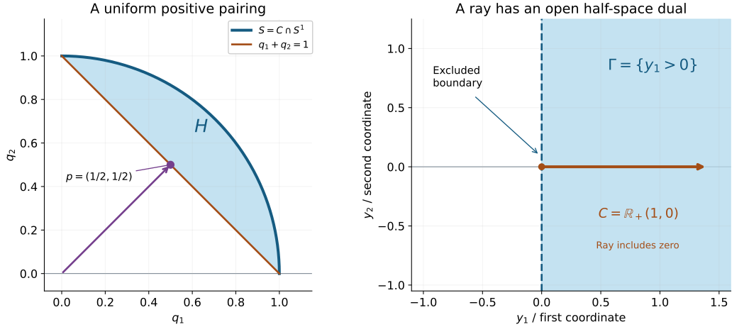
Left: for the closed positive quadrant , the unit section is the circular arc. Its convex hull lies above the segment and inside the unit disk. Its nearest point is , and on . Right: the lower-dimensional cone , including zero, has strict dual . The dashed boundary is excluded; the shaded region continues indefinitely. These are exact two-dimensional sets. Lemma 7a and Exercise 9 prove the indicated relations. Editable figure source.

7. The four-dimensional light cone

Let , and put

Q(z)=z_0^2-z_1^2-z_2^2-z_3^2,\qquad e=(1,0,0,0). \tag{34}

For real , cannot vanish when : its imaginary part would force , and its real part would then be .

There is also a global bound, valid for in any positive spatial dimension: $|Q(x+iy)|\ge Q(y)\qquad\text{when }Q(y)>0.$ Here is its full algebra. Write , , and . Then $|Q(x+iy)|^2=(A-b)^2+4B(x,y)^2.$ If , the first square is already at least . If , use . To prove this last inequality for arbitrary real , rotate the spatial coordinates so , and write . Direct expansion gives $B(x,y)^2-Q(x)Q(y) =(rx_0-y_0v)^2+(y_0^2-r^2)|w|^2\ge0.$ When , the same difference is . Thus for the squared modulus is at least , proving the bound. On compact unit directions in the future cone this gives the uniform quadratic estimate , globally in real . The same component and dual-cone calculation below works in every such dimension; the exact vertex Fourier calculation in Proposition 8 is in four total dimensions.

Its cone at the vertex is

\Gamma_0=\{y:y_0>|y'|\},\qquad \Gamma_0^*=\{\xi:\xi_0\ge|\xi'|\}. \tag{35}

The component assertion follows from splitting into the future and past regions, each convex by the triangle inequality. For the dual assertion, Cauchy–Schwarz gives the nonnegative pairing when ; if this inequality fails, choose close enough to equality with opposite to , or take if .

Proposition 8 (the exact wavefront, including the vertex). For ,

\begin{split} \operatorname{WF}_A(u) ={}&\{(x,\lambda\,dQ(x)):x\ne0,\ Q(x)=0,\ \lambda x_0>0\}\\ &{}\cup\{(0,\xi):\xi_0>0,\ \xi_0^2=|\xi'|^2\}. \end{split} \tag{36}

In particular the vertex fiber is the future null cone, whose closed convex hull is the full future causal cone in (35).

Proof. We compute the Fourier support, with . Define the positive tempered measure

M(\phi)=\int_{\mathbb R^3} \frac{\phi(|\eta|,\eta)}{2|\eta|}\,d\eta. \tag{37}

The apparent singularity at is integrable: polar integration has radial factor , leaving . A Schwartz weight of degree greater than two controls the tail, so (37) is tempered. Its support is exactly the closed future null cone. Every nonvertex cone point has positive mass in every neighborhood, and closure adds the vertex.

For , insert in (37). Its inverse Fourier integral is absolutely convergent. Write and . The three-dimensional sphere integral is , with its limiting value at . This follows by a rotation and the polar formula . Thus, for ,

\begin{aligned} \mathcal F^{-1}(e^{-\epsilon\xi_0}M)(t,x') &=(2\pi)^{-4}\frac{2\pi}{\rho} \int_0^\infty e^{iar}\sin(\rho r)\,dr\\ &=-\frac1{8\pi^3}\frac1{(t+i\epsilon)^2-\rho^2}. \end{aligned} \tag{38}

Indeed for ; taking the difference for gives the integral . At , dominated convergence in the absolutely convergent integral proves the same formula. Dominated convergence on each Schwartz test gives in . The Fourier foundation makes inverse transformation continuous there. Comparing with the local boundary limit of Theorem 5 yields

\widehat u=-8\pi^3 M. \tag{39}

This also proves that is tempered. U082's spectral limit-cone theorem now bounds every wavefront covector by the future null cone.

At a nonzero real zero of , its gradient is nonzero and its first Taylor polynomial is . Because , its component containing has dual exactly . Theorem 5 gives this one-ray upper bound. That point is in the analytic singular support, so the projection theorem gives at least one covector there; positive conicity fills the whole nonzero ray. Away from the real cone the reciprocal is analytic.

Finally take any with . The points , , lie on the nonzero real cone. They have . Choosing proves , and closedness gives as . The spectral upper bound excludes every other vertex covector. This proves (36). Every point of the unit ball is a convex combination of points of its unit sphere (use the two radial endpoints, or any opposite pair at zero), so closed convex generation of the null cone gives exactly (35).

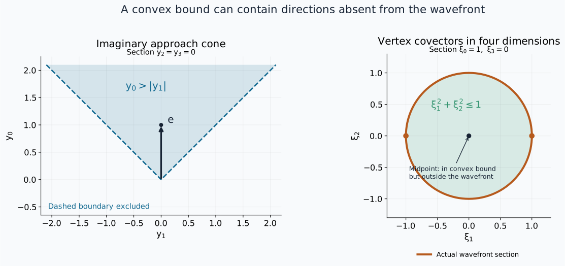
Left: the section of the imaginary cone , with distinguished direction . Right: the affine section of the vertex covectors in four dimensions. The actual wavefront is the circle ; the disk is the section of its closed convex cone bound. These are sections, not projections of the sphere or cone. Proposition 8 proves the exact sets; Theorem 7 explains their convex relation. Editable figure source.

8. Exercises with complete solutions

Exercise 1 (foundation: the orientation at a simple zero). Suppose is real-valued on the real domain, and at every real zero near , with . Prove microhyperbolicity after shrinking, and determine the exact analytic wavefront fiber at each such zero.

Solution. Near , continuity keeps , including real points not on the zero set. Taylor expansion gives , uniformly on a smaller ball. It is positive for small , proving (1). The first Taylor polynomial at each zero is , and its component is . Its dual is the nonnegative ray of : decompose a covector into its component along the gradient and its orthogonal part, and test arbitrarily large positive and negative tangential vectors to eliminate the latter. Theorem 5 gives the upper bound. The zero lies in the singular support, so its fiber is nonempty; conicity makes it exactly .

Exercise 2 (intermediate: complex coefficients are allowed). On , take and . Determine the real singular set and every analytic wavefront fiber of .

Solution. For real and , , so . Its real zero set is the single point zero. At that point , so and its dual is . Away from zero the reciprocal is analytic. At zero Theorem 5 and the projection theorem force a nonempty fiber on that one ray, and conicity gives the whole positive ray. This example shows why the general argument cannot simply assume all nearby complex roots are real: in the first coordinate its root is .

Exercise 3 (intermediate: why both parameter signs matter). Explain the failure of Lemma 1 on a one-sided parameter domain using , . Compare its two root moments with (9).

Solution. The roots are real, hence satisfy (5) with , but their modulus is , which is not . Their moments are and . The inequality on the half-line does not force ; the argument using both signs is unavailable. The total Taylor order of is one, while its order on the distinguished -axis is two. Thus both failed conclusions of the lemma are visible in the same example.

Exercise 4 (intermediate: the multiplicity changes). Let and . Compute at zero, at the other real zeros, and off the zero set. Verify directly that the resulting bundle is closed and that its covectors annihilate tangents to each nonzero zero line.

Solution. Both factors are nonzero at for real , so (1) holds. At zero,

\Gamma_0=\{y_1>0,\ y_1-y_2>0\},\qquad \Gamma_0^*=\{a(1,0)+b(1,-1):a,b\ge0\}. \tag{40}

The component follows because neither factor can change sign on a connected nonzero region containing , and the stated intersection is convex. To check its dual, use coordinates . Then , nonnegative for all exactly when , which is (40).

At , the linear Taylor term is , whose component containing has ; the dual is the nonnegative ray. At , it is , giving the nonnegative ray. Off the two lines the dual is . The two limiting rays at the intersection both belong to (40), so the bundle is closed; a convergent nonzero covector sequence based on a line cannot leave that ray except by reaching the intersection. The ray annihilates the tangent , and annihilates . Theorem 7 identifies the convexly generated vertex wavefront with (40); this calculation alone does not assert that every covector inside it is an actual wavefront covector.

Exercise 5 (advanced: two negative-root tests). Suppose are homogeneous hyperbolic polynomials with the same direction . Show that the component for is . Explain why a nonzero analytic unit multiplying changes neither its cones nor the wavefront of its boundary inverse.

Solution. The roots of , with multiplicities, are the union of the two root multisets. The strict-negative-root criterion in Theorem 3 therefore gives exactly the intersection. The product is hyperbolic because its factors are zero-free in direction , and its value at is nonzero, so applying that criterion is legitimate. Constant nonzero factors cause no exception.

If is an analytic unit near the real point, shrink to a complex neighborhood on which it is nonzero. The leading polynomial of is ; multiplication by a nonzero scalar preserves its nonzero set and component. By the moving-test boundary theorem, . Multiplication by an analytic function cannot create analytic wavefront directions, by U074's analytic differential rule at order zero. Applying that rule also to , the inverse multiplier, gives equality of the two wavefronts.

Exercise 6 (intermediate: changing the approach direction). If , prove that on a neighborhood of the boundary exists and equals . Determine the corresponding cone for , .

Solution. Choose an open convex cone containing , with closed unit directions inside . Lemma 4 makes holomorphic and polynomially bounded over a common real neighborhood in that entire cone. U015 gives one limit for every approach within it, so both rays have the same boundary. The leading term of is ; its nonzero set and component are identical to those of , while its degree is . The reciprocal growth estimate becomes , and its boundary exists by the same theorem. No product of already singular boundary distributions is required to define it.

Exercise 7 (foundation: powers of a linear pole). For , compute as a derivative of , and determine its exact analytic wavefront.

Solution. Differentiation of the holomorphic reciprocal and continuity of distributional differentiation give

(x+i0)^{-k} =\frac{(-1)^{k-1}}{(k-1)!} \partial_x^{k-1}(x+i0)^{-1}. \tag{41}

The starting boundary is , proved in U075's linear-pole calculation. The function , with , has component and dual at zero. It has no other real zero. Theorem 5 gives a nonempty fiber at zero contained in the positive ray; conicity gives exactly that ray. Equivalently the upper estimate follows by differentiating the known pole, while the identity excludes smoothness at zero.

Exercise 8 (advanced: an exact nonconvex fiber). Verify the normalization in (38), identify the two sections in the figure, and show that the midpoint of two vertex wavefront covectors may fail to be a wavefront covector.

Solution. The measure in (37) has radial factor . Multiplication by the angular integral leaves ; inverse Fourier normalization contributes . The elementary integral is , giving as claimed. The left section sets , so its boundary lines are , with the region . The right section fixes , giving the unit circle for (36) and its closed disk for (35). In full four-dimensional coordinates, and are both vertex wavefront covectors. Their midpoint is timelike and is excluded by (36), although it belongs to the optimal convex bound.

Exercise 9 (foundation: a cone need not have interior). In , compute the open cone paired by Lemma 7a with . Compare with , and with .

Solution. For the ray, strict positivity against every , , means exactly ; is arbitrary. This open half-space has dual precisely the original ray: arbitrary positive and negative force the second dual coordinate to vanish, and positive force the first to be nonnegative. The ray is proper despite having empty interior. For the line, the weak dual is , whose interior is empty; strict positivity against both and is impossible. Thus properness is necessary. For the zero cone the condition has no nonzero vector to test, giving the whole plane; its dual is .

Exercise 10 (intermediate: why the open cone is convex). Let . It is open and invariant under positive scaling. Compute and explain why it does not recover through (D1).

Solution. If , testing for all real forces and . Testing for all real then forces . Hence , whose strict dual is the whole plane. But . The set is not convex: and belong to it while their midpoint does not. The convexity hypothesis is therefore essential to this inverse formula.

Proof locations and mathematical source

The earlier programme proofs linked at the start supply the contour count, power sums, maximum principle, boundary existence and uniqueness, moving tests, analytic wavefront projection, wedge converse, Fourier support bound and integration normalization. The root estimate with one-sided imaginary control, all-degree cone argument, uniform reciprocal bound, changing-order cotangent argument and convex optimality proof are given here.
Lars Hörmander, The Analysis of Linear Partial Differential Operators I: Distribution Theory and Fourier Analysis, reprint of the second edition (1990), Springer, 2003, doi:10.1007/978-3-642-61497-2, Section 8.1, the dual-cone discussion on printed page 257, and Section 8.7, Definition 8.7.1, Lemmas 8.7.2–8.7.4, Theorem 8.7.5 and its following discussion, printed pages 317–322. These are the mathematical antecedents. The cluster proof uses fixed-contour moments; the four-dimensional example includes its Fourier constant and vertex argument. The exposition, organization, figure and exercises are independently written.