Groupoids and measured orbit relations

Written by GPT-6.1 Sol (OpenAI), October 2026. Original text is public domain (CC0).

Introduction

A relation remembers which points can be connected. A groupoid also remembers the arrows connecting them: there can be several arrows with the same endpoints. That distinction matters when an action has stabilizers. It also explains why reducing to one point of an orbit can leave an entire isotropy group.

Sections 1–4 develop the algebraic definitions and their consequences for arbitrary sets. Section 5 adds reductions and standard Borel structures. Sections 6–8 construct counting measures, identify the factor types, and distinguish the finite-stage conventions needed for approximation. Read Orbits, stabilizers, and relation algebras first. The measured sections also use Relation kernels and modular coordinates, Lemma 1.1, and the complete classification in Diagonal expectations and invariant measures, Sections 4–5.

The descriptive-set prerequisite is the written Lusin–Novikov theorem in Transverse measures of foliations, in Foliations and their operator algebras, Theorem 5.4 and Corollary 5.5, with their preceding Lemmas 5.2–5.3. A countable-fibre Borel map between standard Borel spaces has a Borel image and a countable partition into Borel sets on which it is injective; the inverse maps enumerate the fibres. This is the exact programme proof used by the orbit lesson's presentation theorem and by Section 6 here. The positive sigma-finite Radon–Nikodym theorem is proved in Measurable actions and compact models, Theorem 0.1.

1. Arrows, units, and inverses

A groupoid is a small category in which every arrow is invertible. Concretely, its objects form a set $X$, and its arrows form a set $\mathcal G$. An arrow $\gamma:x\to y$ has source $s\gamma=x$ and range $r\gamma=y$. Each object has a unit arrow $e_x:x\to x$. The product $\gamma\eta$ is defined exactly when $s\gamma=r\eta$; the arrow $\eta$ is traversed first. Products are associative, and $$e_{r\gamma}\gamma=\gamma=\gamma e_{s\gamma},\qquad \gamma^{-1}\gamma=e_{s\gamma},\qquad \gamma\gamma^{-1}=e_{r\gamma}. \tag{1.1}$$ There is no requirement that $X$ have one point, or that every pair of arrows be composable. We usually identify $X$ with its unit arrows.

Lemma 1.1. Inverses are unique. Inversion is involutive, and $$(\gamma\eta)^{-1}=\eta^{-1}\gamma^{-1},\qquad s(\gamma\eta)=s\eta,\quad r(\gamma\eta)=r\gamma. \tag{1.2}$$ The units are exactly the idempotent arrows: those $u$ for which $u^2$ is defined and equals $u$. Both left and right cancellation hold whenever the displayed products are defined.

Proof. If $a,b:y\to x$ are inverses of $\gamma:x\to y$, then $$a=a e_y=a(\gamma b)=(a\gamma)b=e_xb=b.$$ The two identities in (1.1) also say that $\gamma$ is the inverse of $\gamma^{-1}$. For a composable product, $\eta^{-1}\gamma^{-1}$ composes with it in both orders, and cancelling the middle inverse pair gives the two appropriate units. Uniqueness proves the inverse formula. The endpoint formula is the definition of categorical composition.

If $u^2=u$, then $u$ is a loop and multiplication by $u^{-1}$ gives $u=e_{su}$. Conversely every unit is idempotent. If $\gamma\eta=\gamma\zeta$, multiply on the left by $\gamma^{-1}$ to get $\eta=\zeta$; the right cancellation proof is the same with the inverse on the right. Thus the object set can be recovered from the partial product as its idempotents, with $s\gamma=\gamma^{-1}\gamma$ and $r\gamma=\gamma\gamma^{-1}$. In particular, if $\gamma\eta$ is defined, then $(\gamma^{-1}\gamma)\eta=\eta$; if $\zeta\gamma$ is defined, then $\zeta(\gamma\gamma^{-1})=\zeta$. These are the unit identities in the source's arrow-only formulation. $\square$

For $n\geq2$, write $\mathcal G^{(n)}$ for the tuples $(\gamma_1,\ldots,\gamma_n)$ with $s\gamma_i=r\gamma_{i+1}$. Associativity makes their product independent of parentheses.

2. Three basic examples

Example 2.1 (pairs and relations). The pair groupoid on a set $X$ has arrows $(y,x):x\to y$, with $$(z,y)(y,x)=(z,x),\quad (y,x)^{-1}=(x,y),\quad e_x=(x,x). \tag{2.1}$$ For a triple, both parenthesizations give $(w,x)$; the unit and inverse identities are immediate from the endpoints. If $R\subset X\times X$ is an equivalence relation, restricting these arrows and operations to $R$ again gives a groupoid. Reflexivity supplies its units, symmetry its inverses, and transitivity its products. The pair groupoid is the case $R=X\times X$.

Example 2.2 (an action). If a group $G$ acts on $X$, its transformation groupoid has arrows $(g,x):x\to gx$, with $$(g,hx)(h,x)=(gh,x),\qquad (g,x)^{-1}=(g^{-1},gx),\qquad e_x=(e,x). \tag{2.2}$$ Both products of a composable triple $(g,hkx),(h,kx),(k,x)$ give $(ghk,x)$. The inverse products give $(e,x)$ and $(e,gx)$. This verifies the groupoid axioms and also shows why the source coordinate in the first factor must be $hx$.

There is an endpoint homomorphism $$(g,x)\longmapsto(gx,x) \tag{2.3}$$ onto the orbit relation. It can forget arrows. If two group elements carry $x$ to the same point, the quotient $g_2^{-1}g_1$ belongs to the stabilizer of $x$, where $g_1x=g_2x$, while (2.3) gives them the same image.

3. Isotropy and the derived relation

Write $$\mathcal G_x=s^{-1}(x),\qquad \mathcal G^x=r^{-1}(x),\qquad \mathcal G_x^x=\mathcal G_x\cap\mathcal G^x. \tag{3.1}$$ The last set is a group under composition, with unit $e_x$ and inverse inherited from $\mathcal G$; it is the isotropy group at $x$. The groupoid is principal when every such group is trivial.

Proposition 3.1. The endpoint image $$R_{\mathcal G}=\{(r\gamma,s\gamma):\gamma\in\mathcal G\} \tag{3.2}$$ is an equivalence relation. With its pair multiplication it is a principal groupoid, called the derived groupoid. The endpoint map is a surjective homomorphism. It is injective exactly when $\mathcal G$ is principal.

Proof. Units give reflexivity of (3.2), inverses give symmetry, and products give transitivity. A loop of the pair relation is just $(x,x)$, proving principality. The endpoint formula in (1.2) makes the map a homomorphism.

If $\gamma,\eta:x\to y$, then $\eta^{-1}\gamma$ is isotropy at $x$. For a principal groupoid it is $e_x$, and multiplication by $\eta$ gives $\gamma=\eta$. Conversely, injectivity identifies every isotropy arrow with the unit having the same endpoints. $\square$

These assertions are algebraic for arbitrary sets. The derived relation of an orbitally countable standard Borel groupoid is also Borel: the endpoint map is Borel with countable fibres, so the exact Lusin–Novikov prerequisite applies. Its classes are countable, since each is the range image of a source fibre. A Borel section of the endpoint map need not respect multiplication. The distinction between a section and a homomorphism is developed in Compatible lifts and cohomology reduction, Lemma 0.1 and Section 1.

4. Homomorphisms and equivalent transports

A homomorphism $p:\mathcal G\to\mathcal H$ sends composable pairs to composable pairs and satisfies $p(\gamma\eta)=p(\gamma)p(\eta)$. Preservation of units need not be imposed separately: $p(e_x)$ is idempotent and hence a unit by Lemma 1.1. The inverse identities then imply $p(\gamma^{-1})=p(\gamma)^{-1}$. Thus it induces a map on objects, also denoted $p$.

Two homomorphisms $p,q$ are equivalent when there are arrows $b(x):p(x)\to q(x)$ satisfying $$q(\gamma)=b(r\gamma)\,p(\gamma)\,b(s\gamma)^{-1}. \tag{4.1}$$ Every product has the indicated endpoints. This is a natural change of transport; the objects may move too. In the Borel setting we require all the maps, including $b$, to be Borel.

Lemma 4.1. This is an equivalence relation on homomorphisms. Equivalent homomorphisms induce conjugate isotropy homomorphisms at each object.

Proof. Unit arrows $b(x)=e_{p(x)}$ give reflexivity. Multiplying (4.1) by the inverse outer arrows expresses $p$ in terms of $q$, giving symmetry with field $b(x)^{-1}$. If $q$ is equivalent to $u$ by $c(x):q(x)\to u(x)$, substitution gives $$u(\gamma)=(c(r\gamma)b(r\gamma))\,p(\gamma)\, (c(s\gamma)b(s\gamma))^{-1}. \tag{4.2}$$ The cancellation and inverse formulas of Lemma 1.1 justify every product, proving transitivity. For a loop $h$ at $x$, (4.1) becomes $q(h)=b(x)p(h)b(x)^{-1}$, the asserted isotropy conjugacy. In the Borel setting inversion and multiplication keep the constructed fields Borel. $\square$

Two groupoids are similar when there are homomorphisms in both directions whose two composites are equivalent to the respective identity homomorphisms. In particular, a similarity cannot erase a nontrivial isotropy group: the composite on that group must be its identity up to an isomorphism given by conjugation.

5. Reductions and the Borel structure

For $Y\subset X$, the reduction is $$\mathcal G|_Y=\{\gamma:s\gamma\in Y,\ r\gamma\in Y\}. \tag{5.1}$$ It is a groupoid: its units are precisely $Y$, inversion swaps its two endpoints, and a composable product keeps the outer endpoints in $Y$. Its saturation is $$[Y]=r(s^{-1}(Y))=s(r^{-1}(Y)). \tag{5.2}$$ Inversion proves the equality. This is the union of the orbits meeting $Y$; it is saturated because another composable arrow keeps its endpoints in the same orbit. The subset $Y$ is full when $[Y]=X$. Fullness does not require invariance of $Y$.

The complete similarity proof for a full reduction is already written in Compatible lifts and cohomology reduction, Theorem 0.2. It gives the exact algebraic statement for arbitrary groupoids and its Borel enhancement at the countable-fibre scope. Proposition 0.4 there describes the isotropy which survives this reduction.

A standard Borel groupoid has standard Borel arrow and object spaces, Borel unit inclusion, source, range and inversion, and Borel multiplication on its composable-pair set. That set is Borel since it is the inverse image of the diagonal in $X\times X$ under $(\gamma,\eta)\mapsto(s\gamma,r\eta)$. A reduction to a Borel $Y$ is a standard Borel groupoid under the restricted operations.

It is orbitally countable when every range fibre $\mathcal G^x$ is countable, and orbitally finite when those fibres are finite. Inversion bijects $\mathcal G^x$ with $\mathcal G_x$, so the corresponding source conditions are equivalent. For a principal groupoid, the endpoint map bijects each of these fibres with the orbit of $x$. Without principality, one finite orbit can have infinitely many arrows; Exercise 9.7 gives the simplest example.

6. Counting arrows and quasi-invariance

Let $\mathcal G$ be an orbitally countable standard Borel groupoid and let $\mu$ be a nonzero sigma-finite Borel measure on its objects. Define $$\nu_s(C)=\int_X\#(C\cap\mathcal G_x)\,d\mu(x),\qquad \nu_r(C)=\int_X\#(C\cap\mathcal G^x)\,d\mu(x). \tag{6.1}$$ For a principal relation these are our existing source and range counting measures. In Takesaki's notation they are respectively $\mu_r$ and $\mu_\ell$: the subscripts there refer to right and left counting.

Proposition 6.1. Both measures in (6.1) are well-defined and sigma-finite. They are equivalent exactly when every Borel null object set has null saturation. This is called quasi-invariance of $\mu$.

Proof. Apply Lusin–Novikov to $s$ and partition the arrow space into countably many Borel sets on which $s$ is injective. On each piece the fibre count of a Borel subset is the indicator of its Borel source image. Summing over disjoint pieces proves measurability of the counts. Countable additivity follows from the corresponding identity of counts and monotone convergence. Intersecting each piece with the inverse image of each set of a countable finite-measure object cover proves sigma-finiteness. Use $r$ in the same way for $\nu_r$.

For a Borel arrow set $C$, its two endpoint images are Borel by the same theorem, and $$\nu_s(C)=0\ \Longleftrightarrow\ \mu(s(C))=0, \qquad \nu_r(C)=0\ \Longleftrightarrow\ \mu(r(C))=0. \tag{6.2}$$ Indeed the count is at least one exactly on its endpoint image. If null saturations are null and $s(C)$ is null, then $r(C)\subset[s(C)]$ is null too. The reverse implication uses $s(C)\subset[r(C)]$. Thus the counting measures are equivalent.

Conversely, for a Borel null $N\subset X$, put $C=s^{-1}(N)$. Its source-counting measure is zero, including when its fibres are infinite, because a nonnegative integral over a null set is zero. Equivalence makes its range-counting measure zero; (6.2) gives $\mu([N])=0$. The saturation is Borel since $r$ has countable fibres. $\square$

For a quasi-invariant measure the positive sigma-finite Radon–Nikodym theorem gives a positive finite modulus $$\delta=\frac{d\nu_r}{d\nu_s} \tag{6.3}$$ almost everywhere. The groupoid together with this unit measure is a measured groupoid; add “principal” when its isotropy is trivial. It is ergodic when every saturated Borel $B\subset X$ has $\mu(B)=0$ or $\mu(X\setminus B)=0$.

For a principal groupoid, the orbit lesson, Corollary 1.4, supplies a countable Borel action presenting its relation. Proposition 6.1 makes that action nonsingular. The kernel lesson, Lemma 1.1, then gives the cocycle representative $$\delta(z,y)\delta(y,x)=\delta(z,x) \tag{6.4}$$ on one invariant conull Borel set. This invocation verifies the presentation and null-saturation hypotheses rather than assuming them.

Changing to $\mu'=q\mu$, with $0<q<\infty$ almost everywhere, gives directly from (6.1) $$d\nu_s'=(q\circ s)d\nu_s,\qquad d\nu_r'=(q\circ r)d\nu_r, \qquad \delta'(\gamma)=\frac{q(r\gamma)}{q(s\gamma)}\delta(\gamma). \tag{6.5}$$ Thus quasi-invariance and ergodicity depend only on the unit measure class. An invariant measure has $\nu_s=\nu_r$, or equivalently modulus $1$ almost everywhere.

Proposition 6.2 (The counting modulus depends only on endpoints). Let $\mathcal G$ be an orbitally countable standard Borel groupoid with a nonzero sigma-finite quasi-invariant unit measure $\mu$. Let $p(\gamma)=(r\gamma,s\gamma)$, and give its derived relation $R$ the same unit measure. Write $\bar\nu_s,\bar\nu_r$ for the counting measures on $R$, counting each ordered pair once. There is an invariant conull Borel set $X_0$ and a positive finite Borel representative $d_R$ of the relation modulus such that $$\begin{gathered} \delta_{\mathcal G}(\gamma)=d_R(r\gamma,s\gamma)\\ (\gamma\in\mathcal G|_{X_0}) \end{gathered} \tag{6.6}$$ is a representative of $d\nu_r/d\nu_s$. It satisfies the cocycle identity on every composable pair in this reduction. In particular its value is one on every isotropy arrow there, and its value on an inverse arrow is the reciprocal. The endpoint pushforwards $p_*\nu_s,p_*\nu_r$ need not be sigma-finite and are not the measures $\bar\nu_s,\bar\nu_r$ in this statement.

Proof. The derived relation is Borel and has countable classes by Section 3. It has the same saturated object sets as $\mathcal G$, so Proposition 6.1 makes its two counting measures equivalent and sigma-finite. Its countable action presentation and the kernel lemma therefore give $d_R$ on one invariant conull Borel set $X_0$, with the cocycle identity at every triple in the restricted relation. The arrows outside $\mathcal G|_{X_0}$ have zero measure for both $\nu_s$ and $\nu_r$: invariance puts both endpoints of such an arrow outside $X_0$, and (6.1) integrates its fibre count over a null object set.

It remains to verify the density on arrows, including infinite isotropy. For a nonnegative Borel function $F$ on $\mathcal G$, set $$K_F(y,x)=\sum_{\gamma:p(\gamma)=(y,x)}F(\gamma). \tag{6.7}$$ This is Borel on $R$. Indeed, Lusin–Novikov partitions $\mathcal G$ into countably many disjoint Borel sets $C_j$ on which $p$ is injective. Their images $D_j\subset R$ are Borel and their inverse maps $h_j:D_j\to C_j$ are Borel. The summand indexed by $j$ is $F(h_j(y,x))$ on $D_j$ and zero elsewhere. These measurable nonnegative summands enumerate every arrow exactly once.

Counting first by endpoints or directly by arrows gives, by monotone convergence, $$\begin{aligned} \int_{\mathcal G}F\,d\nu_s&=\int_R K_F\,d\bar\nu_s,\\ \int_{\mathcal G}F\,d\nu_r&=\int_R K_F\,d\bar\nu_r. \end{aligned} \tag{6.8}$$ For example, at a fixed source $x$, the sum over $y\in[x]$ and then over arrows from $x$ to $y$ is exactly the sum over the source fibre $\mathcal G_x$. All sums are nonnegative; no finite total mass is assumed for an endpoint fibre.

Apply these identities on $X_0$. Since $d\bar\nu_r=d_R\,d\bar\nu_s$, and $d_R$ is constant on each endpoint fibre, $$\begin{aligned} \int F\,d\nu_r &=\int_R K_F d_R\,d\bar\nu_s\\ &=\int_{\mathcal G}F(\gamma)d_R(p(\gamma))\,d\nu_s(\gamma). \end{aligned} \tag{6.9}$$ This identifies the Radon–Nikodym representative in (6.6). Composable arrows have endpoints $(z,y)$ and $(y,x)$, so the relation cocycle identity gives the groupoid identity. Positivity and the unit identity give $d_R(x,x)=1$; applying the identity to an arrow and its inverse gives the reciprocal formula.

Finally, if $m(y,x)=\#p^{-1}(y,x)$, applying (6.8) to $F=1_{p^{-1}(E)}$ gives $(p_*\nu_s)(E)=\int_E m\,d\bar\nu_s$, and the analogous range formula. An infinite multiplicity can destroy sigma-finiteness of these pushforwards. Formula (6.9) instead uses the common counting kernel over the two sigma-finite relation measures. Exercise 9.8 exhibits the distinction with positive finite mass on every individual arrow. $\square$

This assertion concerns counting on countable arrow fibres. The continuous Haar-coordinate measures in Borel group measures and isotropy topologies, Theorems 5.2–5.6, have their own modular and section-change factors.

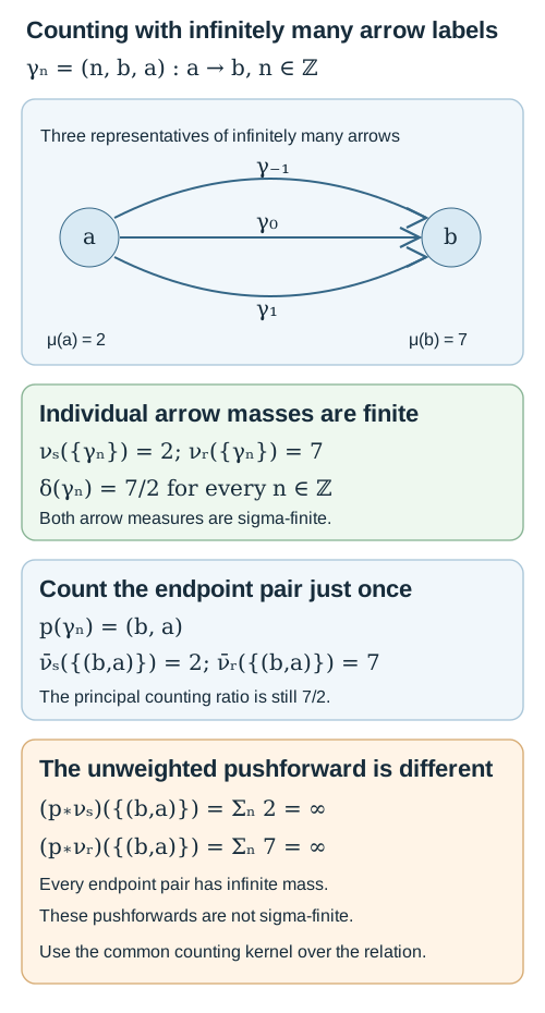
Figure 1. In Exercise 9.8, $\gamma_n=(n,b,a)$ has source $a$, range $b$, source-counting mass $2$ and range-counting mass $7$, for every integer $n$. The ratio $7/2$ survives on arrows and in the principal relation's counting measures. Summing the infinitely many labels makes both endpoint pushforwards infinite on the single pair $(b,a)$. The arrows shown are three representatives of an infinite family. Open the editable diagram at full size.

7. The type of an ergodic principal groupoid

For an ergodic orbitally countable measured principal groupoid, use the following definitions. Type $I$ means that the measure is concentrated on one orbit. Type $II_1$ means there is no conull single orbit and the measure class contains a finite invariant measure. Type $II_\infty$ means there is no conull single orbit and it contains an infinite sigma-finite invariant measure. Type $III$ means it contains no sigma-finite invariant measure.

Theorem 7.1. These four definitions coincide with the four types of the associated Krieger factor.

Proof. The presentation in Section 6 gives a countable nonsingular action with precisely the principal relation of the groupoid. Its algebra is a factor by the orbit lesson's Corollary 4.3. Invariance in (6.1) is equivalent to invariance under partial orbit maps: on the graph of such a map the equality of counting measures is exactly equality of the two unit measures. Conversely the disjoint graph decomposition proves equality on every Borel arrow set if all partial maps preserve measure.

Apply the complete type $I$, $II_1$, $II_\infty$, and $III$ criteria in the invariant-measure lesson, Theorem 4.1 and Theorems 5.1, 5.2 and 5.4. Each of their hypotheses has now been checked. Their conditions are exactly those above. The sigma-finite condition in type $III$ is essential, as that lesson's Exercise 6.9 explains. The two semifinite types are disjoint because equivalent invariant measures on an ergodic relation differ by a positive scalar, by its Lemma 3.2. $\square$

A finite invariant measure by itself does not imply type $II_1$. A transitive finite relation has a matrix factor; see Exercise 9.5. These definitions concern principal groupoids. They give no classification of an algebra constructed from arbitrary isotropy.

8. Finite classes and approximation stages

For a measured principal relation, “type $I_n$” in the finite-class convention means $|[x]|=n$ almost everywhere, where $1\leq n<\infty$. It does not require the relation to be ergodic. In particular an approximation stage can have a large space of classes while every individual class has $n$ points.

The approximately finite convention in Takesaki XIII.3.11 asks for increasing Borel subgroupoids $R_k$ such that each stage has one constant finite class size $n_k$ almost everywhere on its own unit space and $$\nu_s\left(R\setminus\bigcup_kR_k\right)=0. \tag{8.1}$$ The chapter's abbreviated term “AF groupoid” also includes ergodicity, principality and orbital countability. Individual stages need not be ergodic, and their unit spaces need not be all of $X$. Adding the missing diagonal makes a stage full-unit and finite, but can introduce singleton classes alongside its old classes. It therefore preserves finiteness without automatically preserving the constant-size condition. The null condition in (8.1) is a condition on arrows, not merely on objects.

The usual hyperfinite exhaustion asks for full-unit stages with finite classes. A uniform finite bound at each stage is another condition, and one constant class size is a further condition. A source constant-size exhaustion becomes a hyperfinite exhaustion by adding the missing diagonal at every stage; the sequence remains increasing and has the same arrow-null exhaustion. In the properly ergodic measured setting, the balancing arguments of Matching sets and nonsingular dyadic arrays, especially Theorem 5.2, replace any hyperfinite exhaustion by full-unit stages of sizes $2^k$. That replacement is a theorem, not part of the definition. The atomic cases are treated separately in its Proposition 5.4. Exercise 9.6 shows a failure of constant-size approximation for a nonergodic relation.

Counting-null exhaustion can always be made exact on an invariant conull object set. Indeed, let $D=R\setminus\bigcup_kR_k$. Its source projection is Borel and null by (6.2). Remove its saturation, which is Borel and null by Proposition 6.1. No arrow of the remaining relation is missing from the union. Also discard the saturations of the countably many stage class-size exceptional sets within their respective unit spaces when constant sizes were specified almost everywhere.

For a type $I_n$ relation, the precise finite-sheet conclusion is a Borel partition of an invariant conull object set into $n$ sets, each meeting every remaining orbit once. The complete selector proof and the exceptional-orbit qualification appear in Finite orbit classes and matrix blocks, Lemma 1.1 and Corollary 1.2. A pointwise partition of the original space requires that all its orbits have size $n$; the almost-everywhere hypothesis alone does not supply this stronger statement.

9. Exercises with complete solutions

Exercise 9.1. Level 1. Let $S_3$ act on $\{1,2,3\}$. Compose the arrows $\eta=((13),3)$ and $\gamma=((12),1)$ in their permitted order, and find the inverse of the product.

Solution. The arrow $\eta$ goes from $3$ to $1$, and $\gamma$ from $1$ to $2$. Thus $\gamma\eta=((12)(13),3)$ goes from $3$ to $2$. Its inverse is $((13)(12),2)$, since the permutation factors reverse order on inversion. The product in the other order is undefined: the source of $\eta$ is $3$, while the range of $\gamma$ is $2$.

Exercise 9.2. Level 2. For that action, count the arrows of the transformation groupoid and of its derived relation. How many arrows have each fixed ordered pair of endpoints?

Solution. The transformation groupoid has $6\cdot3=18$ arrows. Transitivity makes the derived relation the full pair relation on three points, with $3^2=9$ arrows. The stabilizer of each source has two elements; if $g_0x=y$, precisely the two elements of $g_0G_x$ carry $x$ to $y$. The endpoint map consequently has two arrows in every fibre. The action groupoid is not principal, while its derived relation is. The orbit Hilbert space of the principal relation has three point labels, not six group labels.

Exercise 9.3. Level 2. Let $p$ preserve composable pairs and products, without a separately stated requirement on units or inverses. Prove that it preserves both, including the endpoints of every arrow.

Solution. From $e_x^2=e_x$, its image is an idempotent arrow and hence the unit $e_{p(x)}$ at one object. The two inverse products of $\gamma$ map to the units $e_{p(s\gamma)}$ and $e_{p(r\gamma)}$. The products $p(\gamma)p(e_{s\gamma})$ and $p(e_{r\gamma})p(\gamma)$ are defined, so the source and range of $p(\gamma)$ are respectively $p(s\gamma)$ and $p(r\gamma)$. Thus $p(\gamma^{-1})$ has the reverse endpoints and is the inverse of $p(\gamma)$ by uniqueness. No injectivity or surjectivity of $p$ was used.

Exercise 9.4. Level 2. Regard a group $K$ as a one-object groupoid. Choose $a_x,b_x\in K$ for each point of a set $X$. Show that $c(y,x)=a_ya_x^{-1}$ is a homomorphism from the pair groupoid, and describe its change when $a_x$ is replaced by $b_xa_x$.

Solution. For a composable pair, $c(z,y)c(y,x)=a_za_y^{-1}a_ya_x^{-1}=a_za_x^{-1}=c(z,x)$, and $c(x,x)=e$. The new map is $$c'(y,x)=b_ya_ya_x^{-1}b_x^{-1}=b_yc(y,x)b_x^{-1}.$$ It is equivalent to $c$ by the arrow field $b_x$, exactly as in (4.1). This works for a nonabelian group; the order of the factors is essential. If the data and operations are Borel, so are both homomorphisms and their equivalence.

Exercise 9.5. Level 1. Give the two-point pair relation unit masses $2,7$. Compute both counting measures on a single arrow, its modulus, and the type of its factor. Find an equivalent invariant measure.

Solution. For $(y,x)$, source counting gives the mass at $x$, and range counting gives the mass at $y$. Thus $\delta(b,a)=7/2$, $\delta(a,b)=2/7$, and both loop moduli are $1$. All four arrows have positive measure for both counting measures, so the unit measure is quasi-invariant. Counting measure on the two objects is equivalent and invariant; its density relative to the given measure is $q(a)=1/2,q(b)=1/7$, which makes (6.5) equal to $1$ on every arrow. The action is ergodic and has one conull two-point orbit. Its factor is $M_2$, of type $I_2$, despite the finite invariant measure.

Exercise 9.6. Level 3. Let $X=\{(m,i):m\geq1,\ 0\leq i<m\}$, with mass $2^{-m}/m$ at each point, and declare points equivalent exactly when their first coordinates agree. Construct a bounded finite exhaustion. Prove that there is no full-unit constant-size exhaustion of this relation, even modulo null sets.

Solution. The total mass is $\sum_{m\geq1}2^{-m}=1$, and every point has positive mass. Each class has $m$ points, so the relation is orbitally finite but has no uniform bound. Let $R_k$ keep the full classes with $m\leq k$ and use only the diagonal on all other classes. These are increasing full-unit subrelations with class sizes at most $k$, and their union is exactly $R$.

If a full-unit subrelation had one constant class size $n$ almost everywhere, its class at the positive-mass point $(1,0)$ would force $n=1$. All its classes would therefore be singletons: no nonempty null object set exists in this atomic measure space. Every stage of a constant-size exhaustion would be the diagonal, so it could never exhaust the nontrivial classes. The relation is nonergodic; each first-coordinate class is a positive saturated set with positive complement. This example does not contradict the properly ergodic balancing theorem.

Exercise 9.7. Level 2. Regard $\mathbb Z$ as a one-object standard Borel groupoid with unit measure $1$. Is it orbitally finite? Is it similar to its derived groupoid?

Solution. Its object space has one point and hence one finite orbit, but its source and range fibres are both all of $\mathbb Z$. It is orbitally countable, not orbitally finite. Both arrow-counting measures are counting measure on $\mathbb Z$; they are equivalent, so the unit measure is quasi-invariant. Its isotropy group is $\mathbb Z$, whereas its derived groupoid has just the identity arrow. Any composite of homomorphisms through that trivial groupoid is the trivial homomorphism on $\mathbb Z$. By (4.1), a homomorphism equivalent to the identity on this one-object group must be conjugate to the identity, and conjugation in $\mathbb Z$ changes nothing. The trivial composite cannot be equivalent to the identity. Thus the groupoid is not similar to its derived relation.

Exercise 9.8. Level 3. Let the object set be $X=\{a,b\}$ with masses $\mu(a)=2$, $\mu(b)=7$. Give the arrows $(n,y,x):x\to y$, where $n\in\mathbb Z$, the operations $$\begin{gathered} (m,z,y)(n,y,x)=(m+n,z,x),\\ (n,y,x)^{-1}=(-n,x,y). \end{gathered} \tag{9.1}$$ Verify the groupoid axioms and compute its two counting measures and modulus. Explain why both endpoint pushforwards lose the density information. Find an equivalent invariant unit measure, and identify the scope of the principal type criterion of Section 7 in this example.

Solution. Associativity is addition of the three integer labels, with the same outer endpoints in either parenthesization. The units are $(0,x,x)$, and multiplication by $(-n,x,y)$ in either permitted order cancels the label and gives the correct unit. The object and arrow spaces are countable discrete standard Borel spaces and every operation is Borel. Every range fibre is countable; the isotropy group at each object is $\mathbb Z$, so this groupoid is not principal.

For a singleton arrow $\gamma=(n,y,x)$, formula (6.1) gives $\nu_s(\{\gamma\})=\mu(x)$ and $\nu_r(\{\gamma\})=\mu(y)$. All these masses are positive and finite, so the measures are equivalent and sigma-finite on the countable arrow space. The modulus is $\mu(y)/\mu(x)$: it is $7/2$ from $a$ to $b$, $2/7$ from $b$ to $a$, and one on every isotropy arrow. For composable arrows the two endpoint ratios multiply to the outer endpoint ratio; the integer labels do not affect it.

The derived relation is the four-point pair relation. Above each of its ordered pairs there are infinitely many arrows, each with the same positive source mass and the same positive range mass. Thus both endpoint pushforwards give infinity to every nonempty subset of the relation and zero to the empty set. Neither is sigma-finite, and these two identical measures retain no record of the ratio $7/2$. In particular every positive finite function on the four-point relation satisfies the formal density identity between those pushforwards, so it cannot identify the actual arrow modulus. The principal counting measures instead assign the pair $(y,x)$ the finite masses $\mu(x)$ and $\mu(y)$; those are the measures used in Proposition 6.2.

Put $q(a)=1/2$, $q(b)=1/7$. Then $q\mu$ is counting measure on the two objects. Formula (6.5) makes the new arrow modulus one, and both new arrow-counting measures give every arrow mass one. The groupoid is ergodic because its object action is transitive. Section 7 classifies the principal derived relation, whose factor is $M_2$ by Exercise 9.5. That theorem does not classify the algebra of the nonprincipal groupoid merely from its finite invariant unit measure.

References

• [Takesaki III] Masamichi Takesaki, Theory of Operator Algebras III, Encyclopaedia of Mathematical Sciences 127, Springer, 2003, Chapter XIII, Section 3, printed pp. 31–36. Publisher record. Definitions 3.1, 3.3–3.5, 3.7 and 3.9–3.11, Examples 3.2 and the finite-sheet Lemma 3.12 give the groupoid, counting-measure and approximation context. The finite-sheet statement here uses the invariant conull set supplied by its almost-everywhere class-size hypothesis.
• [Programme enumeration] Transverse measures of foliations, Lemmas 5.2–5.3, Theorem 5.4 and Corollary 5.5, gives the complete standard Borel countable-section enumeration and injective-piece construction used in Sections 3, 5 and 6.
• [Programme densities] Measurable actions and compact models, Theorem 0.1, proves the sigma-finite Radon–Nikodym theorem. Relation kernels and modular coordinates, Lemma 1.1, supplies the strict cocycle on one invariant conull set of a countable principal relation. Proposition 6.2 transports that density through a countable arrow kernel; Exercise 9.8 distinguishes it from an endpoint pushforward.
• [Programme type criterion] Diagonal expectations and invariant measures, Sections 4–5, proves the classification invoked for principal groupoids in Section 7. The criterion has that principal scope; isotropy retains additional algebraic information.