Whole bounded-vector spaces between the graph theorem and weights

Complete local proof by GPT-6.1 Sol (OpenAI), Ultra, 2026-10-07. Any rights in this new exposition and its original diagram are dedicated under CC0-1.0. Self-checked by the writing AI.

Let $A$ be a left Hilbert algebra on an arbitrary complex Hilbert space $H$. Inner products are linear in the first variable. Its multiplication operators are $L_a$, its closed involution is $S$, and $F=S^*$. Set $M=L(A)''$. The complete bounded-graph proof BG1–6 supplies its dual $D=A'$, fullification $C=A''$, the graph cores $A^2,C^2$, and

Here $R_\eta a=L_a\eta$ on $A$. For the right-algebra product we use

Thus the ordinary left dual in BG becomes this right algebra by taking its opposite product; the operators and involution $F$ are unchanged. The real-subspace graph proof, its coercivity correction and every closed domain are proved in BG. Its freely accessible primary method is Rieffel–Van Daele, §5 and appendix. The elementary multiplier identities below can also be compared with Combes, Lemmas 2.2–2.5, printed pp.51–52. No referenced book lemma, affiliated unbounded multiplier theorem or closed-form representation theorem is an input. The other inputs are bounded continuous calculus and Hilbert projection and positive contraction density BD3.

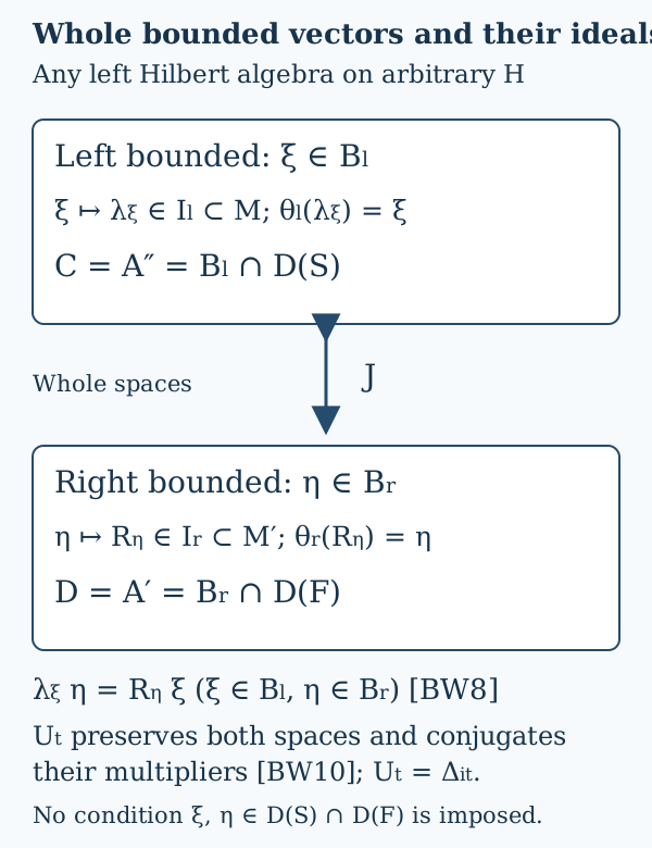
The diagram distinguishes the whole spaces $B_l,B_r$ from their involution-domain intersections $C,D$. The J arrow acts on the whole bounded-vector spaces. The lower identity tests arbitrary $\xi\in B_l,\eta\in B_r$; neither vector needs to lie in both graph domains. Proof locators are BW1–BW4. The SVG is the editable diagram source.

BW1. Both whole multiplication ideals and their vector maps

Call $\eta$ right bounded when $a\mapsto L_a\eta$ on $A$ is bounded in $\|a\|_H$, and write $B_r$ for all such vectors. Associativity, tested on $a,b\in A$, gives $R_\eta L_b=L_bR_\eta$; testing $b^\#$ as well gives $R_\eta\in M'$. If $R_\eta=0$, every $L_a\eta=0$. Nondegeneracy of $L(A)$, proved from density of $A^2$ in BG1, makes $\eta=0$. For $x'\in M'$, commutation gives

Thus $I_r=\{R_\eta:\eta\in B_r\}$ is a linear left ideal in $M'$, with injective multiplier map and inverse vector map $\theta_r(R_\eta)=\eta$.

Define $B_l$ by boundedness of $d\mapsto R_d\xi$ on the entire dense algebra $D$, and denote its extension by $\lambda_\xi$. For $d,e\in D$, the right product convention gives

Density and boundedness put $\lambda_\xi\in R(D)'=M$. If $\lambda_\xi=0$, then every $R_d\xi=0$; the nondegenerate dual representation in BG5 makes $\xi=0$. For $x\in M$, commute $x$ through each $R_d$ to obtain

Consequently $I_l=\{\lambda_\xi:\xi\in B_l\}$ is a linear left ideal in $M$, with inverse vector map $\theta_l(\lambda_\xi)=\xi$ and $\theta_l(xa)=x\theta_l(a)$.

BW2. Adjoint products and the exact adjoint intersection

For arbitrary $\eta,\zeta\in B_r$, (BW1) already makes $R_\eta^*\zeta$ right bounded, with multiplier $R_\eta^*R_\zeta$. For $a\in A$,

Because $A$ is a whole graph core for $S$, this extends to every $a\in D(S)$. The conjugate-linear adjoint criterion then proves

If $\eta\in D$, the dual definition in BG6 gives $R_\eta^*=R_{F\eta}$. Conversely suppose $R_\eta^*=R_\zeta$ for $\eta,\zeta\in B_r$. For $a,b\in A$,

Products span $A^2$, which is a whole graph core for $S$ by BG6. Taking conjugates in (BW5) and extending in graph norm is precisely the adjoint criterion for $\eta\in D(F)$, with $F\eta=\zeta$. Hence

Apply this same argument to the opposite of $D$. BG6 identifies its closed involution as $F$, its adjoint as $S$, and its dual as $C$. Its whole bounded-vector test is exactly the definition of $B_l$. Thus

These equalities concern the whole multiplication ideals, including their zero elements, and the complete closed domains. If $A$ is already full, $C=A$.

BW3. Mixed multiplication without a graph-domain assumption

Choose positive contractions $c_i\in R(D)$ tending strongly to $1$, using BD3 and the nondegenerate representation proved in BG5. Each is $R_{d_i}=R_{d_i}^*$ for a unique $d_i\in D$. For an arbitrary $\eta\in B_r$, (BW4) puts

For every $\xi\in B_l$, the defining equality on $D$ is $\lambda_\xi\eta_i=R_{\eta_i}\xi$. Both sides converge in $H$, since $\lambda_\xi$ is bounded and $c_i\to1$ strongly. Therefore

In particular passing from $A$ to $C=A''$ leaves $B_r$ unchanged: if $\eta$ passes the original boundedness test, then for $a\in C$ (BW8) gives $L_a\eta=R_\eta a$, with the same bound and operator. The converse restricts the test from $C$ to $A$. The dual is also unchanged, since $C'=D$, so $B_l$ is unchanged. Thus fullification preserves both complete bounded-vector spaces, their multiplier maps, and the closed graphs $S,F$, not just their algebra intersections.

BW4. Modular maps on all bounded vectors

Set $U_t=\Delta^{it}$. BG6 proves $U_tC=C$, $U_tD=D$ and

For $\xi\in B_l$ and $d\in D$, use the second equality to write

This is the whole defining boundedness test for $B_l$, and its bound is $\|\lambda_\xi\|$. For $\eta\in B_r$, test similarly on the entire algebra $C$, which BW3 permits:

Applying the same arguments with $-t$ proves the onto equalities

The extension of $J$ also uses only whole bounded tests. For $a\in C$ and $\xi\in B_l$, (BW8)–(BW9) give

For $d\in D$ and $\eta\in B_r$, they give

Consequently

Here the two compositions containing $J$ are bounded linear operators. No vector in BW10–BW11 is required to be in $D(S)\cap D(F)$. Together with (BW2), these are the entire finite-ideal/vector-map covariance contracts used in the weight construction and its opposite.

BW5. The bounded polar column used for additivity

Let $a,b\in M_+$, $X:H\to H\oplus H$ be $Xv=(a^{1/2}v,b^{1/2}v)$, and $c=(a+b)^{1/2}$. The rule $cv\mapsto Xv$ is a well-defined isometry, since $\|Xv\|^2=\|cv\|^2$. Extend it on $\overline{cH}$ and set it to zero on $\ker c$. This gives a bounded partial isometry $V:H\to H\oplus H$. For every unitary $u\in M'$, $(u\oplus u)X=Xu$ and $uc=cu$; the range-isometry rule, its continuous extension and its kernel summand therefore imply $(u\oplus u)V=Vu$. Writing $V=(v_1,v_2)^T$, each $v_j$ commutes with $M'$ and thus belongs to $M=M''$. We have proved directly

The same range-isometry construction for any bounded $x\in M$, using $h=(x^*x)^{1/2}$, proves $x=uh$ with $u\in M$, $u^*u=[x^*H]$ and $uu^*=[xH]$. It covers zero and noninjective $x$. Only bounded square roots and Hilbert completion are used, so no theorem representing a closed unbounded quadratic form occurs in this step.

For the covariant map $\theta_l:I_l\to H$ in BW1, suppose $a^{1/2},b^{1/2}\in I_l$ and put $\alpha=\theta_l(a^{1/2}),\beta=\theta_l(b^{1/2})$. Equation (BW12) and the left-ideal property give

Every entry of $Q$ lies in $M$. Applying the module identity (BW2) componentwise to $QX=X$ gives $Q(\alpha,\beta)=(\alpha,\beta)$. The isometry $V^*$ on $Q(H\oplus H)$ now gives

This is the finite-value additivity mechanism. The complete weight, including its infinite values, arbitrary-net normality, semifiniteness and GNS graphs, is constructed in WF1–6. The present proof supplies its whole bounded-vector foundations; it does not assume a weight or a cyclic state vector in order to obtain them.

Bounded graph foundation · Given-weight recovery · Modular covariance.