The random matrix predictions and their evidence
Written by GPT-6.1 Sol (OpenAI), with contributions by GPT-6 Astra (OpenAI), in Codex at Ultra, October 2026. Original exposition: public domain (CC0).
Two different comparisons with unitary matrices concern the zeta function. One predicts the arrangement of its zeros after rescaling to mean spacing one. The other predicts the growth of its moments on the critical line. The first comparison is local in the zeros; the second includes an arithmetic factor built from primes. Their agreement in several proved cases is evidence for the predictions, rather than a proof of all of them.
We use the Fourier convention \(\widehat r(\alpha)=\int_{\mathbb R}r(u)e^{-2\pi i\alpha u}\,du\), Haar probability measure on \(U(N)\), and \[ K(u)=\frac{\sin\pi u}{\pi u},\qquad K(0)=1. \] The preceding lesson supplies Montgomery's theorem and its precise conjectural extensions. Section 8.1 proves the second moment, including its constant term. The fourth moment is Theorem 6.1 of Mean values of Dirichlet polynomials and zeta. For the matrix calculation, Corollary 4.4 of The Weyl integration formula gives the joint density of labelled eigenangles for Haar probability measure on \(U(N)\): \[ \frac1{N!(2\pi)^N}\prod_{i<j}|e^{i\theta_i}-e^{i\theta_j}|^2. \tag{0.1} \] The normalization includes the labeling convention. On the diagonal torus, conjugation sends the matrix unit \(E_{jk}\) to \(e^{i(\theta_j-\theta_k)}E_{jk}\). Thus the positive-root factors are \(|e^{i\theta_j}-e^{i\theta_k}|^2\), the Weyl group is \(S_N\), and probability measure on the torus is \((2\pi)^{-N}d\theta_1\cdots d\theta_N\). Theorem 3.1, with Lemmas 1.4 and 2.1, proves the Jacobian formula, the \(N!\)-sheeted covering on the regular set, and that the omitted singular set has measure zero. These facts give (0.1), including its factor \(1/N!\). A deterministic ordering instead places the angles in one ordered chamber and multiplies the density there by \(N!\); here the labels are uniformly randomized over all orderings. This also covers \(N=1\), with empty root product and uniform angle. The independent torus-Fourier normalization is written in Exercise 2 of that lesson.
Everything we derive from this density, including the limiting kernel, gap distribution and characteristic-polynomial moments, is proved below.
1. The diagonal and the sine kernel
The function \(K\) is the inverse Fourier transform of the indicator of \([-1/2,1/2]\), by direct integration. Multiplication of these two inverse transforms gives \[ \widehat{K^2}(\alpha)=(1-|\alpha|)_+. \tag{1.1} \] For example, justify the exchange against a Schwartz test function: the two frequency intervals are bounded and the inverse transform of the test is integrable. The convolution of their indicators measures the length of intersection of two unit intervals, which is the triangle in (1.1).
The constant function has Fourier transform \(\delta_0\) as a tempered distribution, while \(\widehat{\delta_0}=1\). Consequently \[ \mathcal F\{\delta_0+1-K^2\} =\delta_0+1-(1-|\alpha|)_+ =\delta_0+\min(|\alpha|,1). \tag{1.2} \] All three expressions are distributions; the delta cannot be treated as an ordinary function at zero.
The diagonal of an ordered pair sum gives the delta on the left. Distinct points in the sine-kernel process have pair density \(1-K(u)^2\). Montgomery's theorem proves the \(|\alpha|<1\) part of the Fourier-side profile, including the narrow spike whose mass becomes the delta. The preceding lesson distinguishes weak convergence of the pair measure from the stronger uniform pointwise Fourier conjecture.
Since \(K(u)=1-\pi^2u^2/6+O(u^4)\), the distinct-pair density vanishes as \(\pi^2u^2/3\) at a collision. This is quadratic repulsion. A nearest-neighbour gap law requires more information: it must exclude all intervening points, not merely count a pair.
2. Unitary matrices give a determinant
The circular unitary ensemble, or CUE, is Haar-random \(U\in U(N)\). Write its eigenvalues as \(e^{i\theta_j}\). With \[ \phi_j(\theta)=\frac{e^{ij\theta}}{\sqrt{2\pi}},\qquad \mathcal K_N(\theta,\varphi)=\sum_{j=0}^{N-1} \phi_j(\theta)\overline{\phi_j(\varphi)}, \] the density (0.1) is \(N!^{-1}\det[\mathcal K_N(\theta_i,\theta_j)]_{i,j=1}^N\). This follows by multiplying the Vandermonde determinant by its conjugate.
Here is the integration identity behind all the correlation functions. For any orthonormal functions \(\phi_0,\ldots,\phi_{N-1}\), Cauchy–Binet gives \[ \det[\mathcal K_N(x_a,x_b)]_{a,b=1}^m =\sum_{\substack{I\subset\{0,\ldots,N-1\}\\ |I|=m}} |\det[\phi_j(x_a)]_{a=1,\ldots,m;\,j\in I}|^2. \tag{2.1} \] Integrate \(x_m\) in each determinant after expanding its last row. Orthogonality removes terms with different last-row indices. Each remaining minor indexed by a set of size \(m-1\) occurs \(N-m+1\) times. Thus the integral of (2.1) is \(N-m+1\) times the determinant for \(m-1\) variables. Iteration, starting at \(m=N\), proves that the density counting ordered distinct \(m\)-tuples is \[ \rho_{N,m}(\theta_1,\ldots,\theta_m) =\det[\mathcal K_N(\theta_i,\theta_j)]_{i,j=1}^m. \tag{2.2} \] In particular its integral is \(N(N-1)\cdots(N-m+1)\), not one.
Unfold the circle by \(\theta=2\pi x/N\); its length is now \(N\), and its one-point density is one. Summing the geometric series in \(\mathcal K_N\), and removing a factor \(e^{i\pi(N-1)(x-y)/N}\) from each kernel entry, gives \[ S_N(x-y)=\frac{\sin\pi(x-y)} {N\sin(\pi(x-y)/N)}. \tag{2.3} \] The phase removal multiplies a determinant's rows and columns by reciprocal factors, so changes no correlation. Removable zeros in this formula are interpreted by the original finite exponential sum.
On each bounded set \(S_N(u)\to K(u)\) uniformly, together with every fixed derivative. Equation (2.2) therefore proves \[ \rho_{N,m}(x_1,\ldots,x_m)\longrightarrow \det[K(x_i-x_j)]_{i,j=1}^m. \tag{2.4} \] For \(m=2\) this is exactly \(1-K(x_1-x_2)^2\). These are matrix theorems, before any conjecture about zeta is made.
3. The same limit in a Gaussian ensemble
The Gaussian unitary ensemble, or GUE, is the probability measure on complex Hermitian matrices \(H\) with density proportional to \(e^{-\operatorname{Tr}H^2}\) with respect to their independent real coordinates. This normalization fixes a scale; unfolding removes it.
Diagonalize \(H=V\operatorname{diag}(\lambda_j)V^*\) away from repeated eigenvalues. In these coordinates \[ dH=V\{d\operatorname{diag}(\lambda)+[A,\operatorname{diag}(\lambda)]\}V^*, \qquad A=V^*dV. \] The invariant Euclidean metric is \(\sum_j d\lambda_j^2+2\sum_{i<j}(\lambda_i-\lambda_j)^2|A_{ij}|^2\). Each off-diagonal entry has two real coordinates. Its volume factor is therefore \((\lambda_i-\lambda_j)^2\), up to a constant. The set of repetitions is the zero set of a nonzero discriminant polynomial and has measure zero. Change of variables gives the eigenvalue density proportional to \[ e^{-\sum_j\lambda_j^2}\prod_{i<j}(\lambda_i-\lambda_j)^2. \tag{3.1} \]
Define the Hermite polynomials by \[ H_n(x)=(-1)^ne^{x^2}\frac{d^n}{dx^n}e^{-x^2},\qquad \varphi_n(x)=\frac{H_n(x)e^{-x^2/2}} {\pi^{1/4}\sqrt{2^n n!}}. \] Integration by parts \(n\) times shows that \(H_n\) is orthogonal to each polynomial of smaller degree for the weight \(e^{-x^2}\). Its leading coefficient is \(2^n\); applying the same calculation to \(H_n\) gives norm \(2^n n!\sqrt\pi\). Hence the \(\varphi_n\) are orthonormal. Factoring their leading coefficients out of a determinant rewrites the normalized version of (3.1) as \(N!^{-1}\det[K_N^{\rm H}(\lambda_i,\lambda_j)]\), where \(K_N^{\rm H}=\sum_{n<N}\varphi_n(x)\varphi_n(y)\). The integration proof in Section 2 applies unchanged.
For clarity, we prove the sine limit at the centre of the Gaussian spectrum. This already explains the common local law in (2.4). Differentiating the defining Hermite formula gives \[ \varphi_n''+(2n+1-x^2)\varphi_n=0,\qquad x\varphi_n=\sqrt{(n+1)/2}\,\varphi_{n+1} +\sqrt{n/2}\,\varphi_{n-1}. \tag{3.2} \] These identities can also be checked by differentiating \(\sum H_n(x)t^n/n!=e^{2xt-t^2}\), obtained by Taylor expansion of \(e^{-(x-t)^2}\). Multiply the recurrence at \(x\) and \(y\), subtract, and telescope to obtain \[ K_N^{\rm H}(x,y)=\sqrt{N/2}\, \frac{\varphi_N(x)\varphi_{N-1}(y) -\varphi_{N-1}(x)\varphi_N(y)}{x-y}. \tag{3.3} \]
Put \(b_N=\pi/\sqrt{2N}\) and \(A_N=(2/(\pi^2N))^{1/4}\). Stirling's formula and the values of \(H_n(0)\) give, for even \(n=2m\), \[ \varphi_{2m}(0)=(-1)^m\pi^{-1/4} \frac{\sqrt{(2m)!}}{2^m m!} =(-1)^m A_{2m}(1+O(m^{-1})). \] Odd values vanish; their derivatives satisfy \(\varphi_{2m+1}'(0)=\sqrt{2(2m+1)}\,\varphi_{2m}(0)\). These initial data and (3.2), after \(x=b_Nu\), imply, uniformly for bounded \(u\) and in the first derivative, \[ \frac{\varphi_n(b_Nu)}{A_N} =\cos(\pi u-n\pi/2)+O_R(N^{-1}), \qquad n=N,N-1,\quad |u|\leq R. \tag{3.4} \] To see the error estimate without invoking an asymptotic formula for orthogonal polynomials, the rescaled differential equation has coefficient \(\pi^2(2n+1)/(2N)-b_N^4u^2=\pi^2+O_R(N^{-1})\). The initial values and first derivatives have the stated relative error. Variation of constants against \(\cos\pi u,\sin\pi u\) gives an error bounded by \(C_R/N+C_R\int_0^{|u|}|{\rm error}(v)|\,dv\); iterating this integral inequality proves (3.4). Differentiating the variation-of-constants expression proves its derivative version.
The numerator of (3.3), divided by \(A_N^2\), now tends to \(\sin\pi(u-v)\) with a uniform first derivative error. Its value on \(u=v\) is identically zero, so division by \(u-v\) is harmless, also on the diagonal. Since \(\sqrt{N/2}A_N^2=1/\pi\), \[ b_N K_N^{\rm H}(b_Nu,b_Nv)\longrightarrow K(u-v) \tag{3.5} \] uniformly on bounded squares. Determinants prove every fixed \(m\)-level limit at the centre. Thus CUE and this Gaussian bulk limit have the same sine-kernel correlations, despite their different global spectra.
The conclusion holds at any fixed point inside the bulk, with its local density used for unfolding. Here are the additional estimates. For \(n=N,N-1\), set \(q_n(x)=2n+1-x^2\) and \(z_n(x)=\int_0^x\sqrt{q_n(t)}\,dt\). On \(|x|\leq c_*\sqrt{2N}\), with fixed \(c_*<1\), the substitution \(\varphi_n=q_n^{-1/4}v_n(z_n)\) in (3.2) gives \[ v_n''+v_n=R_n v_n,\qquad R_n=\frac{q_n''}{4q_n^2}-\frac{5(q_n')^2}{16q_n^3}. \] The bound \(|R_n|\leq C_{c_*}N^{-2}\) holds, and the corresponding \(z_n\)-interval has length \(O(N)\). The exact initial values above, followed by variation of constants, now show \[ v_n(z)=\sqrt{2/\pi}\{\cos(z-n\pi/2)+O_{c_*}(N^{-1})\} \tag{3.6} \] with the same error for \(v_n'\). Indeed the integral equation has kernel \(\sin(z-t)R_n(t)\), whose absolute integral is \(O(N^{-1})\); its iteration bounds \(v_n\) and the error uniformly. This also proves (3.6) for negative \(z\).
Choose \(x_0=c\sqrt{2N}\), \(|c|<1\), and \(b=\pi/\sqrt{2N(1-c^2)}\). Uniformly for bounded \(u\), \[ z_n(x_0+bu)=z_n(x_0)+\pi u+O(N^{-1}),\qquad q_n(x_0+bu)^{-1/4}=(2N(1-c^2))^{-1/4}(1+O(N^{-1})). \] Moreover \[ (z_N(x_0)-N\pi/2)-(z_{N-1}(x_0)-(N-1)\pi/2) =-\arccos c+O(N^{-1}), \] because the difference of the two square roots is \(1/\sqrt{2N-t^2}+O(N^{-3/2})\), uniformly along the integral from \(0\) to \(x_0\). The trigonometric determinant in (3.3) therefore has leading factor \(\sqrt{1-c^2}\sin\pi(u-v)\). Its amplitude, after multiplication by \(\sqrt{N/2}\), is again \(1/\pi\). The errors have uniform first derivatives in \(u,v\), and vanish on the diagonal before division. This proves \[ bK_N^{\rm H}(x_0+bu,x_0+bv)\longrightarrow K(u-v) \tag{3.7} \] uniformly on compact sets, also when \(c\) ranges over a compact subset of \((-1,1)\). Thus the stated \(m\)-level law holds throughout the interior bulk. No claim about the edge, whose scaling and kernel differ, is involved.
4. A gap distribution is a determinant of an operator
For the sine kernel on \((0,s)\), define its Fredholm determinant by the convergent series \[ E(s)=\sum_{m=0}^\infty\frac{(-1)^m}{m!} \int_{(0,s)^m}\det[K(x_i-x_j)]\,dx_1\cdots dx_m. \tag{4.1} \] The matrix in the integrand is a Gram matrix: \(K(x-y)=\int_{-1/2}^{1/2}e^{2\pi i\xi(x-y)}\,d\xi\). Its determinant is nonnegative and at most one by the Gram determinant inequality, as all diagonal entries are one. Absolute convergence follows from \(\sum s^m/m!\).
In finite CUE, inclusion–exclusion for the number of points in \((0,s)\) gives (4.1) with \(S_N\) and \(m\leq N\), provided \(s<N\). Each determinant is again a Gram determinant with diagonal one. Dominated convergence and (2.4) show that the finite probability of an empty interval tends to \(E(s)\). The finite GUE has the same limit by (3.5): on a bounded interval its rescaled diagonal kernel is uniformly bounded, which gives the dominating bound \(C_s^m\) instead of one.
There is also a useful bound at large \(s\). For finite CUE the gap probability is \(\det(I-B)\), where \[ B_{ij}=\int_0^s\phi_i^{\rm unfolded}(x) \overline{\phi_j^{\rm unfolded}(x)}\,dx,\quad 0\leq i,j<N. \] Expand the determinant in principal minors and apply Cauchy–Binet inside their integrals to get the inclusion–exclusion series. The matrix \(B\) is positive, has eigenvalues in \([0,1]\), and has trace \(s\), because it is the restriction of orthonormal functions on the whole circle. Hence \[ 0\leq\det(I-B)\leq e^{-\operatorname{Tr}B}=e^{-s}. \] Passing to the limit gives \(0\leq E(s)\leq e^{-s}\).
The nearest-neighbour spacing density of the limiting unitary law is \[ p(s)=E''(s),\qquad s\geq0. \tag{4.2} \] We justify both the derivative and its probabilistic meaning. For any configuration of \(N\) points on a circle of length \(N\), with cyclic gaps \(\ell_j\), the fraction of starting positions whose following interval of length \(s\) is empty equals \[ \frac1N\sum_{j=1}^N(\ell_j-s)_+. \tag{4.3} \] The CUE law is invariant under rotation, so expectation of (4.3) is its empty-interval probability. Its negative derivative is the expected fraction of gaps exceeding \(s\); its distributional second derivative is the empirical gap probability measure.
To pass derivatives to the limit, rescale each integral in (4.1) to \((0,1)^m\). On any complex disk \(|s|\leq R\), the entries \(K(s(u-v))\), and the finite-sum entries \(S_N(s(u-v))\), are bounded uniformly in \(N,u,v\). Hadamard's inequality bounds the absolute value of a determinant by \(m^{m/2}C_R^m\). The resulting series \(\sum R^m m^{m/2}C_R^m/m!\) converges. Thus the Fredholm series and the finite series converge locally uniformly as entire functions of \(s\); Cauchy's formula gives convergence of derivatives. Formula (4.3) proves that \(p\geq0\) on the real half-line and that it is the limiting gap density.
Equation (4.1) gives \(E(0)=1\) and \(E'(0)=-1\). Convexity, monotonicity and \(E(s)\to0\) imply \(E'(s)\to0\). Therefore \[ \int_0^\infty p(s)\,ds=1,\qquad \int_0^\infty s\,p(s)\,ds=1. \tag{4.4} \] For the second identity integrate by parts; the boundary \(sE'(s)\) vanishes because convexity gives \(|E'(s)|\leq2E(s/2)/s\).
The widely used \(2\times2\) Wigner approximation \[ \frac{32}{\pi^2}s^2e^{-4s^2/\pi} \] is a useful approximation to (4.2), not its definition. The determinant (4.1) includes all the higher correlation functions and is the spacing law used in our numerical comparison.
5. An exterior-power calculation
Let \(Z_U=\det(I-U)\). Its expansion is \[ Z_U=\sum_{j=0}^N(-1)^j\operatorname{tr}(\Lambda^jU). \tag{5.1} \] For a diagonal matrix this is the elementary symmetric-polynomial expansion of the determinant; diagonalization proves it for all unitary matrices.
We verify the representation facts needed to integrate the square. In the wedge basis \(e_{i_1}\wedge\cdots\wedge e_{i_j}\), the diagonal torus acts with distinct weights \(\prod_{i\in I}t_i\). An operator commuting with every diagonal matrix is diagonal in this basis. If it also commutes with the permutation matrices, its diagonal values are equal, because permutations act transitively on the \(j\)-element subsets. Thus its commutant is scalar. A proper invariant subspace of a unitary representation would have a nonscalar orthogonal projection in its commutant. Consequently \(\Lambda^j\mathbb C^N\) is irreducible, including the one-dimensional cases \(j=0,N\). The central matrix \(tI\) acts by \(t^j\), so representations with different \(j\) are inequivalent.
For completeness the character orthogonality follows by Haar averaging. If \(\pi,\sigma\) are irreducible unitary representations, average a linear map \(A\) as \(\int\pi(U)A\sigma(U)^*\,dU\). It is an intertwiner. Its kernel and image are invariant, so it vanishes if the representations are inequivalent. For \(\pi=\sigma\), an intertwiner is scalar: an eigenspace over \(\mathbb C\) of any such map is invariant, which forces the map to be scalar. Taking its trace gives the scalar \(\operatorname{tr}A/\dim\pi\). Apply this to the matrix units; then sum the resulting coefficient identities on the two character diagonals to obtain \[ \int\chi_\pi(U)\overline{\chi_\sigma(U)}\,dU =\begin{cases}1,&\pi\simeq\sigma,\\0,&\pi\not\simeq\sigma.\end{cases} \] Expanding (5.1), therefore, \[ \boxed{\ \mathbb E_{U(N)}|Z_U|^2=N+1.\ } \tag{5.2} \] The \(N+1\) summands are contributions of representations, rather than independent random coefficients.
6. Every unitary moment
For real \(k>-1/2\), Keating and Snaith's exact formula is \[ \mathbb E_{U(N)}|Z_U|^{2k} =\prod_{j=0}^{N-1} \frac{\Gamma(j+1)\Gamma(j+1+2k)}{\Gamma(j+1+k)^2}. \tag{6.1} \] We prove it using a determinant and analytic uniqueness.
First suppose \(k\) is a nonnegative integer. Expanding the two Vandermonde determinants in (0.1) and integrating each variable shows \[ \mathbb E|Z_U|^{2k} =\det[c_{i-j}]_{i,j=0}^{N-1},\qquad c_\ell=\frac1{2\pi}\int_0^{2\pi}|1-e^{i\theta}|^{2k} e^{-i\ell\theta}\,d\theta. \tag{6.2} \] The determinant integration identity used here is direct: for functions \(f_i,g_j\), expand both determinants in permutations to get \(\int\det[f_i(x_j)]\det[g_i(x_j)]\prod_jd\mu(x_j) =N!\det[\int f_i g_j\,d\mu]\). Since \((1-z)^k(1-z^{-1})^k=(-1)^kz^{-k}(1-z)^{2k}\), the Laurent coefficients are \(c_\ell=(-1)^\ell\binom{2k}{k+\ell}\). Removing the row and column signs in (6.2) leaves a binomial determinant.
For integers \(a,b\geq0\), put \[ D_N(a,b)=\det\left[\binom{a+b}{a+i-j}\right]_{i,j=0}^{N-1}, \] where a binomial coefficient outside its range is zero. The evaluation is \[ D_N(a,b)=\prod_{j=0}^{N-1} \frac{j!(a+b+j)!}{(a+j)!(b+j)!}. \tag{6.3} \] Here is an induction that checks every constant. For \(N=0,1\) the formula is immediate. If \(a=0\) or \(b=0\), the matrix is triangular with diagonal one, and the product also equals one. For \(a,b\geq1\), the adjacent-minor identity gives \[ D_N(a,b)D_{N-2}(a,b) =D_{N-1}(a,b)^2 -D_{N-1}(a+1,b-1)D_{N-1}(a-1,b+1). \tag{6.4} \] To verify the identity for an arbitrary matrix, assume its middle \((N-2)\)-square is invertible, take its Schur complement to reduce to a \(2\times2\) determinant, and cancel its determinant. The resulting polynomial identity holds for all matrices by continuity.
Write \(P_n(a,b)\) for the proposed product. Cancelling its factors gives \[ \frac{P_n(a+1,b-1)P_n(a-1,b+1)}{P_n(a,b)^2} =\frac{ab}{(a+n)(b+n)}. \] Also \(P_NP_{N-2}/P_{N-1}^2 =(N-1)(a+b+N-1)/((a+N-1)(b+N-1))\). This is precisely one minus the last displayed ratio for \(n=N-1\). The positive induction value \(D_{N-2}=P_{N-2}\) permits division in (6.4), proving (6.3). Taking \(a=b=k\) proves (6.1) at all nonnegative integers.
To extend the identity, use \(k\) as a complex variable. The integral \[ D(k)=\mathbb E\exp(2k\log|Z_U|) \] is holomorphic for \(\Re k>-1/2\). Indeed (0.1) has a bounded Vandermonde factor, and each possible singularity at \(\theta_j=0\) is dominated on a compact \(k\)-set by an integrable power \(|\theta_j|^{2\sigma}\), with \(\sigma>-1/2\). Logarithmic derivatives are dominated too. The right side \(Q(k)\) of (6.1) is holomorphic and nonzero in the same half-plane.
For \(\sigma=\Re k\geq0\), \(|D(k)|\leq4^{N\sigma}\). Uniform Stirling estimates in the closed right half-plane give \[ Q(k)=C_N4^{Nk}k^{-N^2/2}(1+O_N(|k|^{-1})), \qquad C_N>0,\quad |k|\to\infty,\ \Re k\geq0. \] Thus \(f=D/Q-1\) has at most polynomial growth in that half-plane. Dividing it by a sufficiently high integer power of \(1+k\) makes a bounded holomorphic function on \(\Re k>0\), vanishing at every positive integer.
Such a function must vanish identically. Here is the needed uniqueness fact. Map the half-plane to the disk by \(z=(k-1)/(k+1)\). The zeros at \(k=n\geq2\) become \(z_n=(n-1)/(n+1)\). A bounded nonzero holomorphic function on the disk has \(\sum_n-\log|z_n|<\infty\): factor a possible zero at the centre, apply Jensen's formula on a radius \(r<1\), bound the boundary mean by the logarithm of its supremum, and let \(r\uparrow1\). But \(-\log z_n\geq1-z_n=2/(n+1)\), whose sum diverges. This contradiction proves uniqueness. Hence \(D=Q\) for \(\Re k>0\), and the identity theorem continues the equality to \(\Re k>-1/2\). This proves (6.1), including the integrability range.
7. The Barnes factor and the size of a matrix
The Barnes \(G\)-function can be normalized by the convergent product \[ G(1+z)=(2\pi)^{z/2} \exp\left(-\frac{z+(1+\gamma)z^2}{2}\right) \prod_{n=1}^\infty \left\{(1+z/n)^n\exp\left(\frac{z^2}{2n}-z\right)\right\}. \tag{7.1} \] The logarithm of each product factor is \(O_R(n^{-2})\) on a fixed disk away from its finitely many zeros. The product therefore defines an entire function, with \(G(1)=1\).
We record its recurrence rather than assume its normalization. Let \(L(z)=\log G(1+z)\) on a zero-free region. Differentiation of the convergent product gives \[ L'(z)=\tfrac12\log(2\pi)-\tfrac12-(1+\gamma)z +\sum_{n\geq1}\left(\frac{n}{n+z}-1+\frac zn\right). \tag{7.2} \] Subtract this formula at \(z\) from the formula at \(z+1\). Rearranging the convergent difference, using \[ \frac{-n}{(n+z)(n+z+1)} =-\frac1{n+z+1} +\frac{z}{(n+z)(n+z+1)}, \] and telescoping the second term, gives \(L'(z+1)-L'(z)=\psi(z+1)\), the logarithmic derivative of gamma. The constant is fixed by \(G(2)=1\). To check that value in (7.1), the logarithm of its first \(M\) factors at \(z=1\) is \[ M\log(M+1)-\log M!-M+\tfrac12 H_M \longrightarrow 1-\tfrac12\log(2\pi)+\tfrac12\gamma \] by Stirling's formula and \(H_M=\log M+\gamma+o(1)\). The prefactor in (7.1) has the opposite logarithm. Hence analytic continuation gives \[ G(z+1)=\Gamma(z)G(z). \tag{7.3} \] In particular \(G(1+k)=\prod_{j=0}^{k-1}j!\) for integers \(k\geq1\), and \[ f_k:=\frac{G(1+k)^2}{G(1+2k)} =\prod_{j=0}^{k-1}\frac{j!}{(j+k)!}. \tag{7.4} \]
Applying (7.3) to (6.1) writes the exact moment as \[ \mathbb E|Z_U|^{2k} =f_k\frac{G(N+1)G(N+1+2k)}{G(N+1+k)^2}. \tag{7.5} \] For fixed real \(k>-1/2\), this has the asymptotic \[ \mathbb E|Z_U|^{2k}\sim f_kN^{k^2}. \tag{7.6} \] A second derivative proves it without needing a full asymptotic expansion of \(G\). Differentiating (7.2) once more and using the convergent digamma series gives \[ L''(z)=\psi(z+1)+z\psi'(z+1)-1=\log z+O(z^{-2}) \quad(z\to+\infty). \] The last equality follows from the differentiated Stirling estimates. Therefore \[ L(N+2k)-2L(N+k)+L(N) =\int_0^k\int_0^k L''(N+u+v)\,du\,dv =k^2\log N+O_k(N^{-1}). \] The oriented integrals also apply when \(k<0\). Exponentiation proves (7.6). The matrix predicts a power \(k^2\), with the universal factor \(f_k\).
8. The arithmetic factor and zeta moments
For real \(k\geq0\), define \[ d_k(p^m)=\frac{k(k+1)\cdots(k+m-1)}{m!},\quad d_k(1)=1, \] and \[ a_k=\prod_p(1-p^{-1})^{k^2} \sum_{m=0}^\infty d_k(p^m)^2p^{-m}. \tag{8.1} \] At \(k=0\), the definition gives \(d_0(p^m)=0\) for \(m>0\), so \(a_0=1\). At positive \(k\) it agrees with the gamma quotient in the question. For fixed \(k\), the coefficients grow at most as a fixed power of \(m+1\), by the ratio of successive terms or gamma estimates. The local sum is \(1+k^2/p+O_k(p^{-2})\); multiplication by \((1-1/p)^{k^2}\) cancels the linear term. Its positive factors are \(1+O_k(p^{-2})\), so the product converges to a positive number.
The Keating–Snaith moment conjecture for zeta is \[ \frac1T\int_0^T|\zeta(1/2+it)|^{2k}\,dt \sim a_kf_k(\log T)^{k^2},\qquad k\geq0\text{ fixed}. \tag{8.2} \] The matching size is \(N\sim\log T\): both a unitary spectrum and the zeta zeros near height \(T\) then have the corresponding local density after their natural angular or ordinate scaling. The arithmetic factor is essential. A Haar unitary matrix has no Euler product.
We check the first constants exactly. For \(k=1\), \(d_1(p^m)=1\), the sum in (8.1) is \((1-p^{-1})^{-1}\), and every local factor is one. Thus \(a_1=f_1=1\). For \(k=2\), \(d_2(p^m)=m+1\); differentiation of the geometric series gives \[ \sum_{m\geq0}(m+1)^2x^m=\frac{1+x}{(1-x)^3}. \] Its local factor is \((1-x)^4(1+x)/(1-x)^3=1-x^2\), where \(x=p^{-1}\). The Euler product and the value \(\zeta(2)=\pi^2/6\) give \[ a_2=\frac1{\zeta(2)}=\frac6{\pi^2},\qquad a_2f_2=\frac1{2\pi^2}. \tag{8.3} \] The absolutely convergent Euler product is an input from Dirichlet series and Euler products. One short proof of the special value uses the Fourier series of \(x^2\) on \([-\pi,\pi]\). Two integrations by parts give its constant coefficient \(\pi^2/3\) and cosine coefficients \(4(-1)^n/n^2\). The resulting series converges uniformly and has these Fourier coefficients. It equals \(x^2\): the continuous periodic difference has every Fourier coefficient zero, so its Fejér means vanish and also converge uniformly to the difference. The latter convergence follows directly by writing the Fejér kernel as the square of a finite geometric sum; it has integral one, is nonnegative and tends uniformly to zero outside any fixed neighbourhood of zero. Evaluate at \(x=\pi\) to get \(\pi^2=\pi^2/3+4\sum_{n\geq1}n^{-2}\), as required.
The exact rational values from (7.4) are
| \(k\) | \(f_k\) | \(g_k=(k^2)!\,f_k\) |
|---|---|---|
| 1 | \(1\) | \(1\) |
| 2 | \(1/12\) | \(2\) |
| 3 | \(1/8640\) | \(42\) |
| 4 | \(1/870912000\) | \(24024\) |
For example the third denominator is \(3!\,4!\,5!/(0!\,1!\,2!)=8640\), and the fourth is \(4!\,5!\,6!\,7!/(0!\,1!\,2!\,3!)=870912000\). Division of \(9!\) and \(16!\) by these denominators gives \(42\) and \(24024\). These agree with the sixth- and eighth-moment constants proposed by Conrey–Ghosh and Conrey–Gonek before the general matrix prediction.
The cases \(k=1,2\) of (8.2) are theorems. Their unnormalized statements are \[ \int_0^T|\zeta(1/2+it)|^2\,dt =T\log(T/2\pi)+(2\gamma-1)T+o(T), \tag{8.4} \] and \[ \int_0^T|\zeta(1/2+it)|^4\,dt =\frac{T}{2\pi^2}\log^4T+O(T\log^3T). \tag{8.5} \]
8.1. The second moment with its constant term
We prove the stronger second-moment statement (8.4) here. The written Riemann–Siegel expansion, Theorem 5.4 and its uniform remainder in Lemma 5.3, gives, for sufficiently large \(t\), \[ \begin{aligned} \zeta(1/2+it)&=P(t)+e^{-2i\vartheta(t)}\overline{P(t)}+O(t^{-1/4}),\\ P(t)&=\sum_{n\leq\sqrt{t/(2\pi)}}n^{-1/2-it}. \end{aligned} \tag{8.6} \] Its bounded correction coefficient is absorbed by the displayed error; its removable endpoint values are included in that theorem. Write \(\varphi(t)=\tfrac t2\log(t/(2\pi))-\tfrac t2-\pi/8\). The proved gamma phase estimate, The Gamma function and Stirling's formula, Proposition 5.3, says \(\vartheta(t)-\varphi(t)=O(t^{-1})\).
First integrate \(|P(t)|^2\) on \([t_*,T]\), with fixed sufficiently large \(t_*\). A pair \((m,n)\) occurs for \(t\geq\max(t_*,2\pi m^2,2\pi n^2)\). If \(m<n\), its oscillatory integral has magnitude at most \(2/\log(n/m)\). Put \(M=\lfloor\sqrt{T/(2\pi)}\rfloor\). The sum of these bounds with coefficients is \(O(M\log(2M))\): for \(n/2\leq m<n\), use \(\log(n/m)\geq(n-m)/n\) and \((mn)^{-1/2}\leq\sqrt2/n\); for \(m<n/2\), use \(\log(n/m)\geq\log2\) and \(\sum_{m<n/2}m^{-1/2}\ll\sqrt n\). Thus \[ \begin{aligned} 2\int_{t_*}^T|P(t)|^2dt &=2\int_{t_*}^T H_{\lfloor\sqrt{t/(2\pi)}\rfloor}\,dt+O(\sqrt T\log T)\\ &=T\log(T/(2\pi))+(2\gamma-1)T+O(\sqrt T\log T). \end{aligned} \tag{8.7} \] because \(H_{\lfloor\sqrt{t/(2\pi)}\rfloor}=\tfrac12\log(t/(2\pi))+\gamma+O(t^{-1/2})\).
The cross term in the square of (8.6) is also \(o(T)\). Replace \(e^{2i\vartheta(t)}\) by \(e^{2i\varphi(t)}\); the resulting integral error is at most \(C\int_{t_*}^T|P(t)|^2/t\,dt=O(\log^2 T)\), by (8.7) on dyadic blocks and summation. The phase attached to \((m,n)\) is \[ \begin{aligned} f_{mn}(t)&=2\varphi(t)-t\log(mn),\\ f_{mn}'(t)&=\log\frac{t}{2\pi mn},\\ f_{mn}''(t)&=1/t. \end{aligned} \] Let \(f\) be a real twice continuously differentiable phase whose derivative is monotone and satisfies \(f^{\prime}\geq\lambda>0\). Integration by parts gives \[ \begin{aligned} \int_a^b e^{if(t)}dt&=\left[\frac{e^{if(t)}}{if^{\prime}(t)}\right]_a^b\\ &\quad+\int_a^b\frac{e^{if(t)}f^{\prime\prime}(t)}{i(f^{\prime}(t))^2}dt. \end{aligned} \] The endpoint terms are at most \(2/\lambda\), and monotonicity bounds the integral of \(|f^{\prime\prime}|/(f^{\prime})^2\) by \(1/\lambda\). The same bound applies to a negative monotone derivative bounded away from zero by changing \(f\) to \(-f\).
For \(m<n\), its interval begins at \(t\geq2\pi n^2\), so \(f_{mn}'\geq\log(n/m)>0\). Integration by parts, using the monotonicity of this derivative, gives \(O(1/\log(n/m))\). The same coefficient sum as before is \(O(\sqrt T\log T)\). For \(m=n\), the second-derivative integral test gives \(O(\sqrt T)\), since \(f_{nn}''\geq1/T\). This test follows by bounding the interval where \(|f'|\leq T^{-1/2}\) by its length \(2\sqrt T\) and applying the first-derivative test on its at most two complementary intervals. Summing the diagonal coefficients \(1/n\) gives \(O(\sqrt T\log T)\). Hence the whole cross term has that order.
Finally the error in (8.6) has squared integral \(O(\sqrt T)\). The other two terms have squared norm \(O(T\log T)\), by (8.7) and the preceding cross-term bound. Cauchy–Schwarz therefore bounds the change of squared norms by \(O(T^{3/4}\sqrt{\log T}+\sqrt T)=o(T)\). The fixed initial interval has finite integral. Combining this with (8.7) proves (8.4), with its constant term. The proof uses only the already written Riemann–Siegel argument and gamma phase; no mollifier or spectral prerequisite from the later sections of that lesson is involved.
The fourth-moment formula (8.5) is Theorem 6.1 of the mean-value lesson. Its contour decomposition, averaged remainder bounds and cross-term estimate are supplied there. Both leading terms match (8.2). The general conjecture does not follow by interpolation from these two values or from the exact matrix formula.
9. Restricted higher correlations of zeta zeros
Assume RH. Let \(f(x_1,\ldots,x_n)\) be symmetric and invariant under adding the same number to all its arguments. Suppose \[ f(x)=\int_{\mathbb R^n}\Phi(\xi) \delta(\xi_1+\cdots+\xi_n)e^{2\pi i x\cdot\xi}\,d\xi, \tag{9.1} \] where \(\Phi\) is smooth and compactly supported in \(\sum_j|\xi_j|<2\). The delta specifies the measure: integrate out \(\xi_n=-\sum_{j<n}\xi_j\), without an additional Euclidean surface-measure factor. Put \(L=\log T\), and let \(N_T\) count the zero indices in \([T,2T]\), with multiplicity.
The restricted Rudnick–Sarnak theorem, in its zeta specialization, is \[ \frac1{N_T} \sum_{\substack{\gamma_{j_1},\ldots,\gamma_{j_n}\in[T,2T]\\ j_1,\ldots,j_n\ {\rm distinct}}} f\left(\frac{L\gamma_{j_1}}{2\pi},\ldots, \frac{L\gamma_{j_n}}{2\pi}\right) \longrightarrow \int_{\mathbb R^{n-1}}f(0,u_2,\ldots,u_n) \det[K(u_i-u_j)]_{i,j=1}^n\,du_2\cdots du_n, \quad u_1=0. \tag{9.2} \] Distinct indices are required, rather than an assumption that every zero is simple. The zero count gives \(N_T\sim TL/(2\pi)\).
We prove (9.2) by comparing moments of local counting functions. The finite unitary calculation needed in the comparison is an exact identity. If \(\mu,\nu\) are partitions of integers \(d,e\), respectively, and \(d,e\leq N\), then \[ \mathbb E_{U(N)}p_\mu(U)\overline{p_\nu(U)} =\mathbf1_{\mu=\nu}z_\mu,\qquad p_\mu(U)=\prod_{a\in\mu}\operatorname{Tr}U^a,\quad z_\mu=\prod_{r\geq1}r^{m_r}m_r!. \tag{9.3} \] For \(d\ne e\), central multiplication \(U\mapsto tU\), with \(t\in S^1\), multiplies the integrand by \(t^{d-e}\). Haar invariance leaves its integral unchanged; choosing \(t^{d-e}\ne1\) makes the integral zero. For \(d=e\), use the Frobenius identity \(p_\mu=\sum_{\lambda\vdash d}\chi^\lambda(\mu)s_\lambda\), proved in The symmetric groups III: characters and symmetric functions, Corollary 4.1, equation (34). Here Theorem 3.1 identifies the character labels with the Young-ideal labels, using the proved dominance-cancellation Lemma 2.2; there is no unspecified permutation of the partition labels. Specialization to \(N\) variables kills precisely the Schur functions with \(\ell(\lambda)>N\). The unitary Schur characters for \(U(n)\) and their orthogonality are Theorem 2.2 and equation (2.4) of Unitary groups: characters, dimensions and branching. In particular, they remain continuous at repeated eigenvalues. Applying orthogonality to the two finite Schur expansions gives the exact identity, for every \(N\geq1\) and every common degree \(d\): \[ \begin{aligned} &\mathbb E_{U(N)}p_\mu(U)\overline{p_\nu(U)}\\ &\quad=\sum_{\substack{\lambda\vdash d\\\ell(\lambda)\leq N}} \chi^\lambda(\mu)\overline{\chi^\lambda(\nu)}. \end{aligned} \tag{9.3a} \] All partitions of \(d\leq N\) have length at most \(N\), so none are lost on specialization. Character column orthogonality, Corollary 4.2, for \(S_d\) gives the right side of (9.3). Its preceding Theorem 4.1 proves completeness, so the sum really includes every irreducible character. The cycle-type and centralizer calculation, Proposition 4.2, gives \(|C_{S_d}(\sigma_\mu)|=z_\mu\): a commuting permutation permutes the \(m_r\) cycles of length \(r\) and rotates each independently, giving \(r^{m_r}m_r!\) choices. The character values are real because a permutation and its inverse have the same cycle type, while \(\chi(\sigma^{-1})=\overline{\chi(\sigma)}\); keeping the conjugation in (9.3a) also makes the Hermitian convention explicit. These are written programme proofs, not planned inputs. In terms of labelled factors, (9.3) pairs each positive power with an equal negative power, with a factor equal to that power for each pair. The factorial \(m_r!\) counts its possible pairings.
The stable-range restriction is necessary. For \(N=1\) and \(\mu=\nu=(2)\), one has \(|p_{(2)}(U)|^2=1\), whereas \(z_{(2)}=2\). Formula (9.3a) still holds: only the one-row partition survives. The empty partition has \(p_\varnothing=1\) and \(z_\varnothing=1\), so degree zero is included.
There is also a direct tensor interpretation through Schur–Weyl duality, Theorem 5.1 of the unitary lesson. On \(E=(\mathbb C^N)^{\otimes d}\), define \(P_\sigma(v_1\otimes\cdots\otimes v_d)=v_{\sigma^{-1}(1)}\otimes\cdots\otimes v_{\sigma^{-1}(d)}\). This is a genuine action and commutes with \(U^{\otimes d}\). In the standard tensor basis, the diagonal coefficient of \(U^{\otimes d}P_\sigma\) is \(\prod_j U_{i_j,i_{\sigma^{-1}(j)}}\). Summing the indices around each cycle gives \(\operatorname{Tr}(U^r)\), so \[ \operatorname{Tr}_E(U^{\otimes d}P_\sigma)=p_{\operatorname{type}(\sigma)}(U). \] Taking the same trace on the proved \(U(N)\times S_d\) decomposition gives the Schur expansion and hence (9.3a). For \(N\geq d\) every partition occurs; comparison with the linearly independent Schur characters identifies its multiplicity characters with the same \(\chi^\lambda\). This retains the tensor route alongside the symmetric-function proof, rather than assuming either classification without its proof.
For a Schwartz function \(a\) with smooth compactly supported Fourier transform, define \[ A_a(t)=\sum_\gamma a\left(\frac{L}{2\pi}(\gamma-t)\right). \] The explicit formula of the first lesson, with the gamma estimate near \(t\asymp T\), gives uniformly for \(T\leq t\leq2T\) \[ A_a(t)=\widehat a(0) -\frac1L\sum_{m\geq2}\frac{\Lambda(m)}{\sqrt m} \{\widehat a(\log m/L)m^{-it} +\widehat a(-\log m/L)m^{it}\} +O_a(L^{-1}). \tag{9.4} \] The sum is finite. To verify the uniform error, the archimedean density is \((2\pi)^{-1}\log(t/2\pi)+O(1/t)\); integration against the rescaled \(a\) gives \(\widehat a(0)\log(t/2\pi)/L+O_a(1/(TL))\). Away from \(t\), rapid decay of \(a\) bounds the archimedean tails. The two pole terms evaluate \(a\) at \((L/(2\pi))(\pm i/2-t)\); compact Fourier support and integration by parts make them \(O_a(T^{-B})\) for any prescribed \(B\), after increasing the number of integrations. This proves (9.4).
Choose tests \(a_1,\ldots,a_r\) whose Fourier supports lie in intervals \(I_j\). Write \[ P=\sum_j\max(0,\sup I_j),\qquad M=\sum_j\max(0,-\inf I_j), \] and suppose \(P,M<1-\eta\) for some \(\eta>0\). Expand the product of (9.4), and average over \(t\in[T,2T]\). A chosen positive-frequency product is a Dirichlet polynomial of length at most \(T^P\); a negative-frequency product has length at most \(T^M\). The mean-value inequality from Mean values of Dirichlet polynomials and of zeta on the critical line, polarized between two polynomials, makes the average equal to its equal-integer diagonal plus an error tending to zero.
More explicitly, a product with \(r\) prime-power factors has coefficient bounded by \(C_r d_r(m)(\log m)^r/(\sqrt m L^r)\). For each fixed \(\varepsilon>0\), \(d_r(m)\ll_{r,\varepsilon}m^\varepsilon\): in its Euler product the polynomial in a prime exponent is bounded by \(p^{\varepsilon v}\) uniformly for large primes, and the finitely many smaller primes are absorbed into a constant. Thus \(\sum m|c_m|^2\ll Y^{1+\varepsilon}(\log T)^{C_r}\) for length \(Y\). The polarized error divided by \(T\) is \(O(T^{-1}\sqrt{Y_+^{1+\varepsilon}Y_-^{1+\varepsilon}}(\log T)^{C_r})=o(1)\), on choosing \(\varepsilon\) smaller than the support margin. This also handles unequal numbers of factors and a constant polynomial.
Unique factorization analyzes the diagonal. Its leading contributions match a prime appearing once on each side. For two selected tests, their weight is \[ \frac1{L^2}\sum_p\frac{\log^2p}{p} \widehat a_i(\log p/L)\widehat a_j(-\log p/L) \longrightarrow\int_0^\infty u\widehat a_i(u)\widehat a_j(-u)\,du. \tag{9.5} \] This is partial summation from the prime number theorem: on each bounded support interval the measure \(L^{-2}\sum_p(\log^2p/p)\delta_{\log p/L}\) tends to \(u\,du\). The interval next to zero has mass \(O(\epsilon^2)+o(1)\) up to \(\epsilon\), again by partial summation.
All other diagonal blocks are negligible. If the common total exponent of a prime on each side is \(v\geq2\), its denominator is \(p^v\). Summing the possible prime-power exponents in that block gives a finite bound \[ \sum_p\sum_{v\geq2}\frac{C_r v^{C_r}(\log p)^r}{p^v}<\infty. \] The block has at least two factors and also carries \(L^{-r_{\rm block}}\), so tends to zero. This covers both a higher prime power on each side and repetitions of the same prime. The other, ordinary pair blocks are bounded by (9.5). Removing a distinct-prime restriction from these ordinary blocks changes the answer by the same negligible repeated-prime terms.
It follows that the limiting joint moments of the \(A_{a_j}\) are obtained by choosing singleton factors \(\widehat a_j(0)\) and pairing the remaining factors, each pair contributing \[ C(a_i,a_j)=\int_{\mathbb R}|u| \widehat a_i(u)\widehat a_j(-u)\,du. \tag{9.6} \] The two possible orientations of a prime supply the two half-lines. Signs in (9.4) cancel in each pair. Its \(O(L^{-1})\) errors cause no difficulty. For any selected positive-frequency product, the diagonal calculation just made bounds its squared coefficient sum by a constant: pair blocks are bounded and repeated-prime blocks vanish. Its length is still below \(T^{1-\eta}\), so the mean-value inequality bounds its mean square on the height interval. The same holds for a negative-frequency product. Cauchy–Schwarz bounds the mean absolute value of their product uniformly; multiplying by \(O(L^{-1})\) gives \(o(1)\). There is no need to assume a bound for arbitrarily high moments outside the support range.
The corresponding calculation is exact on the unitary side before taking a limit. Periodize \(a_j\) on a circle of length \(N\). Its sum over unfolded eigenangles is \[ \widehat a_j(0)+\frac1N\sum_{\ell\ne0} \widehat a_j(\ell/N)\operatorname{Tr}U^\ell. \tag{9.7} \] In any product under our support conditions, the sums of positive and negative integer powers are less than \(N\). Identity (9.3) applies. The covariance is \(N^{-2}\sum_{\ell\ne0}|\ell|\widehat a_i(\ell/N)\widehat a_j(-\ell/N)\), which tends to (9.6) by Riemann sums. The full local counting moments of zeta and CUE have the same limits.
We explain how this covers (9.1) and excludes coincidences. A product test corresponds to \[ f_a(x_1,\ldots,x_n)=\int_{\mathbb R}\prod_{j=1}^n a_j(x_j-v)\,dv; \] its transform on \(\sum\xi_j=0\) is \(\prod_j\widehat a_j(\xi_j)\). Every point of the compact support in (9.1) has a rectangular neighbourhood with \(P,M<1-\eta\): on that hyperplane its positive and negative sums are equal and less than one. Use finitely many such neighbourhoods and a smooth partition of unity. Extend \(\Phi\) smoothly off the hyperplane there. On each rectangle a Fourier-series expansion with interior cutoffs expresses it as a convergent sum of separated products. Smoothness makes the expansion coefficients decrease faster than any fixed power of the Fourier-series indices. The preceding bounds use only finitely many supremum and derivative norms of the separated factors, which grow polynomially in those indices. Their products with the expansion coefficients are absolutely summable. Consequently both the error estimates and the diagonal limits pass through the expansion. This proves the comparison for arbitrary \(\Phi\).
For an all-index sum, average \(\prod A_{a_j}(t)\) over \([T,2T]\). The substitution \(v=Lt/(2\pi)\) gives \(2\pi/(TL)\) times its sum of \(f_a\), after localization at the ends. Here are bounds for that step. Let \[ q(u)=K(u)^2+K(u-1/2)^2. \] It satisfies \(c/(1+u^2)\leq q(u)\leq C/(1+u^2)\): off a fixed compact set its two numerators are \(\sin^2\pi u\) and \(\cos^2\pi u\), and on the compact set they have no common zero. For large fixed \(h\), a sufficiently small \(\epsilon>0\) makes the nonnegative function \(q(\epsilon u)^h\) a majorant, up to a constant, of every Schwartz test and each polynomially weighted tail needed here. Its transform is compactly supported in \([-h\epsilon,h\epsilon]\) and has as many continuous derivatives as needed when \(h\) is increased. Choose \(nh\epsilon<1/2\). The same explicit-formula and mean-value proof bounds the average of any product of its local counting sums uniformly.
The bounds also apply to short subintervals of \([T/2,3T]\): the mean-value inequality bounds the integral over a subinterval of length \(H\) by \(C H+O(T^{1-\eta/2})\), with some fixed margin \(\eta>0\) for these majorants. Thus centres within \(R/L\) of either endpoint have contribution \(o(T)\), for fixed \(R\). Elsewhere an external zero or an external centre introduces a test argument of absolute value at least \(R/(2\pi)\). Its Schwartz tail is bounded by \(C_B R^{-B}q(\epsilon u)^h\), so its normalized contribution is \(O_B(R^{-B})\). Centres outside \([T/2,3T]\) are negligible directly by rapid decay and the polynomial zero count; choose the decay power larger than the fixed number of factors. First let \(T\to\infty\), then \(R\to\infty\). This justifies localization, including replacement of all zeros by zero indices in \([T,2T]\). The summable separated expansion transfers the bounds to general \(\Phi\).
Apply now the finite inclusion–exclusion identity over partitions of \(\{1,\ldots,n\}\). Identifying the indices in a block merges its frequencies to \(\eta_B=\sum_{j\in B}\xi_j\). The induced transform is smooth, compactly supported, and satisfies \(\sum_B|\eta_B|<2\). The Möbius coefficient of a partition is \(\prod_B(-1)^{|B|-1}(|B|-1)!\); within any nontrivial coincidence these coefficients sum to zero, by counting permutations according to their cycles and their signs. Thus comparison of all-index sums implies comparison of ordered distinct-index sums. For CUE these converge to the determinant in (2.4). Finally \(N_T\sim TL/(2\pi)\) gives (9.2).
For \(n=3\), write \(f(x)=b(x_1-x_2,x_1-x_3)\). Its frequencies are \((a+b,-a,-b)\); the support condition becomes \[ |a+b|+|a|+|b|<2 \quad\Longleftrightarrow\quad \max(|a|,|b|,|a+b|)<1. \tag{9.8} \] This is the interior of the hexagon with vertices \((1,0),(0,1),(-1,1),(-1,0),(0,-1),(1,-1)\). Expanding the \(3\times3\) determinant gives the density \[ 1-K(u)^2-K(v)^2-K(u-v)^2 +2K(u)K(v)K(u-v). \tag{9.9} \] This proves the leading triple-correlation result in Hejhal's range. His weight \(\prod_{i<j}\exp(-(\gamma_i-\gamma_j)^2/6)\) changes no limit: on bounded unfolded differences it tends uniformly to one, while the same majorants bound the complementary Schwartz tails. For general \(n\), (9.2) is the restricted theorem of Rudnick–Sarnak. Products of primes cease to be shorter than the height interval at the proof's support boundary.
10. Families and the symmetry point
High zeros of one \(L\)-function and low zeros averaged across a family are different statistics. The Katz–Sarnak prediction assigns a family a compact symmetry group, usually unitary, symplectic, or orthogonal. It compares zeros near the central point with eigenangles near \(1\) in that group. Their unitary bulk laws agree away from the symmetry point; their densities at that point differ.
We compute those differences on the matrix side. For Haar \(USp(2g)\), choose the positive eigenangles \(0\leq\theta_j\leq\pi\); the others are their negatives. The normalized symplectic Weyl formula, equation (4.6), with quaternionic rank equal to \(g\), gives density proportional to \[ \prod_{i<j}(\cos\theta_i-\cos\theta_j)^2\prod_j\sin^2\theta_j. \tag{10.1} \] This is the Gram determinant of \(\sqrt{2/\pi}\sin(j\theta)\), \(1\leq j\leq g\), divided by \(g!\). Indeed \(\sin(j\theta)/\sin\theta\) is a polynomial of degree \(j-1\) in \(\cos\theta\) with leading coefficient \(2^{j-1}\), by the sine addition recurrence. Its determinant is a Vandermonde times the sine factors in (10.1). Section 2's integration proof gives the positive-angle correlations.
Unfold near zero by \(\theta=\pi x/g\), \(x\geq0\). Riemann sums give \[ \frac2g\sum_{j=1}^g\sin(\pi jx/g)\sin(\pi jy/g) \longrightarrow K(x-y)-K(x+y). \tag{10.2} \] The one-point density is \(1-K(2x)\).
For \(SO(2g)\), the root factors in the Weyl formula leave weight one and the same Vandermonde in \(\cos\theta\). The orthonormal basis is \(1/\sqrt\pi\), then \(\sqrt{2/\pi}\cos(j\theta)\), \(1\leq j<g\). The same determinant and Riemann-sum argument gives kernel \(K(x-y)+K(x+y)\) and density \(1+K(2x)\). For \(SO(2g+1)\), the extra roots give weight \(1-\cos\theta\); an orthogonal basis is \(\sqrt{2/\pi}\sin((j-1/2)\theta)\), \(1\leq j\leq g\). Division by \(\sin(\theta/2)\) gives successive polynomials in \(\cos\theta\), proving the determinant assertion. Its moving positive angles have kernel \(K(x-y)-K(x+y)\), and there is an eigenvalue \(1\) forced by odd dimension. These calculations use Theorem 3.1 and equations (3.3)–(3.5) of the Weyl-integration lesson and the classical-root and normalizer calculation in RT-CPT-07. The following comparison supplies their normalization and the spectral folding used here.
Orthogonal normalization and spectral folding. We now justify the two orthogonal calculations, including their constants. Fix an integer \(g\geq1\). The torus has rotation angles modulo \(2\pi\), with probability measure \((2\pi)^{-g}d\theta\). In the even case the positive roots are \(\varepsilon_i-\varepsilon_j\) and \(\varepsilon_i+\varepsilon_j\), \(i<j\); in the odd case add \(\varepsilon_i\). These are the defining-weight and exterior-square calculation in the classical-root and normalizer calculation in RT-CPT-07. That calculation also proves that the even normalizer has \(2^{g-1}g!\) elements modulo the torus, whereas the odd one has \(2^g g!\). For \(g=1\), the even group is the torus \(SO(2)\) itself: its root set is empty and its Weyl group is trivial. No rank-one root system of type \(D\) is being assumed.
Put \(D_g(\theta)=\prod_{i<j}(2\cos\theta_i-2\cos\theta_j)\). For each pair of indices, the product of the two positive-root factors is \[ \begin{aligned} &|1-e^{i(\theta_i-\theta_j)}|^2 |1-e^{i(\theta_i+\theta_j)}|^2\\ &\qquad=16\sin^2\frac{\theta_i-\theta_j}{2} \sin^2\frac{\theta_i+\theta_j}{2}\\ &\qquad=(2\cos\theta_i-2\cos\theta_j)^2. \end{aligned} \] The extra odd root contributes \(4\sin^2(\theta_i/2)\). Apply Theorem 3.1 and equations (3.3)–(3.5) of the Weyl-integration lesson to a function of the eigenvalue multiset. Fold each torus angle to \([0,\pi]\). Except on a Lebesgue-null boundary there are \(2^g\) choices of signs; both the root product and this spectral function are unchanged by every such choice. Consequently the joint densities of uniformly randomly labeled positive angles, with respect to \(d\theta_1\cdots d\theta_g\) on \([0,\pi]^g\), are \[ \begin{aligned} &p_{D,g}(\theta) =\frac{2D_g(\theta)^2}{g!(2\pi)^g},\\ &p_{B,g}(\theta) =\frac{D_g(\theta)^2}{g!(2\pi)^g}\\ &\qquad{}\times\prod_{j=1}^g4\sin^2\frac{\theta_j}{2}. \end{aligned} \tag{10.2a} \] The factors follow directly: \(2^g/(2^{g-1}g!)=2/g!\) in even dimension and \(2^g/(2^g g!)=1/g!\) in odd dimension. The symmetric law is identified by its integrals against continuous symmetric tests: any test can first be averaged over permutations, without changing its integral under either randomly labeled law. The normalization in the Weyl provider, applied to the constant function, therefore proves mass one. On an ordered chamber instead, multiply these densities by \(g!\). Repeated angles and endpoints have probability zero under these densities; deterministic ordering there has no effect on the law.
Why the even sign restriction matters. An odd number of sign reversals is not generally realized by conjugation in \(SO(2g)\). For distinct angles in the interior with no root degeneracy, the signed tuples with the same eigenvalue multiset split into two even-sign Weyl orbits, hence can represent two different \(SO(2g)\) conjugacy classes. Our folding computes their common spectral statistic, not a general class function on that group. Using \(2^g\) as though it were the even Weyl-group sign factor would lose the factor two in (10.2a). At \(g=1\) the displayed laws reduce to \(p_{D,1}=1/\pi\) and \(p_{B,1}=2\sin^2(\theta/2)/\pi\), agreeing with this same distinction.
Exact Gram determinants. Define functions on \([0,\pi]\) by \[ \begin{aligned} \phi_0(\theta)&=\pi^{-1/2},\\ \phi_j(\theta)&=\sqrt{2/\pi}\cos(j\theta),\quad 1\leq j<g,\\ \psi_j(\theta)&=\sqrt{2/\pi}\sin((j-\tfrac12)\theta) ,\quad 1\leq j\leq g. \end{aligned} \] Each of these two lists is orthonormal for Lebesgue measure. For the cosine list this follows by integrating the cosine product identity, including the constant function. For the half-sine list the product is half the difference of cosines of integer frequencies \(j-k\) and \(j+k-1\); its integral is zero off the diagonal and \(\pi/2\) before normalization on the diagonal. Thus no nonconstant weight is being inserted into these inner products: the odd density's weight is already contained in the half-sine functions.
To check the determinant constants, let \(T_j(x)=\cos(j\arccos x)\). The recurrence \(T_{j+1}=2xT_j-T_{j-1}\), with \(T_0=1\), \(T_1=x\), shows degree \(j\) and leading coefficient \(2^{j-1}\) for \(j\geq1\). Also put \(Q_{j-1}(\cos\theta)=\sin((j-\tfrac12)\theta)/\sin(\theta/2)\). The initial polynomials are \(Q_0=1\), \(Q_1=1+2x\); the same recurrence gives degree \(j-1\) and leading coefficient \(2^{j-1}\). This identity extends to the endpoints by continuity of the polynomial identity after multiplying by \(\sin(\theta/2)\). A determinant of successive-degree polynomial rows is the product of their leading coefficients times the Vandermonde: eliminating lower-degree terms reduces it to the monomial-row determinant. Its sign depends on the column ordering but disappears on squaring. Applying this calculation, including the displayed normalization factors, gives \[ \begin{aligned} &\bigl(\det[\phi_{i-1}(\theta_j)]_{i,j=1}^g\bigr)^2\\ &\quad=\frac{2}{(2\pi)^g}D_g(\theta)^2,\\ &\bigl(\det[\psi_i(\theta_j)]_{i,j=1}^g\bigr)^2\\ &\quad=\frac{D_g(\theta)^2}{(2\pi)^g} \prod_{j=1}^g4\sin^2\frac{\theta_j}{2}. \end{aligned} \tag{10.2b} \] For example the cosine determinant's squared prefactor relative to the Vandermonde in \(\cos\theta\) is \(2^{(g-1)^2}\pi^{-g}\); the factor in \(D_g^2\) is \(2^{g(g-1)}\). Their quotient is \(2^{1-g}\pi^{-g}\), as in (10.2b). For the odd determinant the leading-coefficient factors already give \(2^{g(g-1)}\), leaving \((2/\pi)^g\prod_j\sin^2(\theta_j/2)\). Both formulas include \(g=1\) with empty products.
It follows that each density in (10.2a) is its squared evaluation determinant divided by \(g!\), or equivalently its Gram determinant divided by \(g!\). Expanding both evaluation determinants and integrating one variable at a time leaves only equal permutations by orthonormality: there are \(g!\), each contributing one. This gives a second normalization check without an unevaluated multiple integral. The determinant integration argument of Section 2 applies to either orthonormal list and yields the positive-angle correlation kernels below, where \(a_j=j-1/2\): \[ \begin{aligned} &L_{D,g}(\theta,\varphi)=\frac1\pi\\ &\quad{}+\frac2\pi\sum_{j=1}^{g-1} \cos(j\theta)\cos(j\varphi),\\ &L_{B,g}(\theta,\varphi)\\ &\quad=\frac2\pi\sum_{j=1}^{g} \sin(a_j\theta)\sin(a_j\varphi). \end{aligned} \tag{10.2c} \]
Scaled kernels and the forced point. Change variables by \(\theta=\pi x/g\). A correlation determinant of order \(k\) picks up \((\pi/g)^k\), so its kernel with respect to \(dx\) is \(\widehat L_{*,g}(x,y)=(\pi/g)L_{*,g}(\pi x/g,\pi y/g)\). The cosine product identity makes the even kernel \(1/g\) plus the sum, divided by \(g\), of \(\cos(\pi j(x-y)/g)+\cos(\pi j(x+y)/g)\), for \(1\leq j<g\). The odd kernel is the analogous difference, at the midpoints \((j-1/2)/g\), \(1\leq j\leq g\). Since \[ \int_0^1\cos(\pi t u)\,dt=K(u),\qquad K(0)=1, \] we obtain \[ \begin{aligned} &\widehat L_{D,g}(x,y)\\ &\;\longrightarrow K(x-y)+K(x+y),\\ &\widehat L_{B,g}(x,y)\\ &\;\longrightarrow K(x-y)-K(x+y). \end{aligned} \tag{10.2d} \] These limits are uniform on every compact subset of \([0,\infty)^2\). Indeed for \(0\leq x,y\leq R\), each integrand in the Riemann sums has absolute value at most one and derivative in \(t\) at most \(2\pi R\). On each interval of length \(1/g\), comparing its integral with an endpoint or midpoint value bounds the error by \(2\pi R/g^2\). Summing the errors gives \(O_R(1/g)\); the missing endpoints and the even constant term also contribute \(O(1/g)\). This proves the uniform assertion directly. Determinants, being finite polynomials in the entries, then converge for every fixed order of positive-angle correlation.
On the diagonal the limits are \(1+K(2x)\) and \(1-K(2x)\). All moving eigenangles occur in conjugate pairs, so their one-level intensities on the negative axis are the reflections of these positive-axis intensities. An element of \(SO(2g+1)\) has a forced eigenvalue \(+1\): its nonreal eigenvalues pair up, its \(-1\) eigenvalues have even multiplicity because the determinant is one, and the remaining odd real multiplicity therefore includes \(+1\). In the torus parametrization there is exactly one distinguished fixed \(+1\); any additional endpoint eigenvalues form a null event for (10.2a). It contributes one atom at zero after scaling, not two. Compact-uniform convergence of the moving diagonal kernels gives convergence against compactly supported continuous tests after reflection, and the fixed atom is unchanged. This proves precisely the full-line one-level profiles stated next.
The resulting full-line one-level profiles are \[ \begin{array}{c|c} \text{unitary}&1\\ \text{symplectic}&1-K(2x)\\ \text{even orthogonal}&1+K(2x)\\ \text{odd orthogonal}&1-K(2x)+\delta_0\\ \text{equal mixture of orthogonal types}&1+\tfrac12\delta_0 . \end{array} \tag{10.3} \] The noncentral profiles are reflected evenly from \(x>0\), and the scale counts both halves of the spectrum. A forced eigenvalue is counted once. The central point detects symmetry information absent from the bulk pair law. These are locally finite intensity measures, not probability measures on the whole line: convergence is tested against compactly supported continuous functions. The last row means an equal mixture of the preceding two limiting orthogonal profiles. Identifying it with any particular finite-dimensional disconnected orthogonal-group ensemble requires a separate treatment of that ensemble’s determinant components; no such identification is used here.
These compact symmetry groups should be distinguished from the Gaussian orthogonal and symplectic ensembles in the quantum-chaos conjecture. In the compact groups just calculated, all positive-angle kernels have the unitary bulk limit: at any fixed \(0<\theta_0<\pi\), put \(\theta=\theta_0+\pi x/g\) in the finite sine or cosine sums. The angle-difference term is a Riemann sum tending to \(K(x-y)\); the angle-sum term is a geometric sum bounded by \(C_{\theta_0}\), hence tends to zero after division by \(g\). The constant and half-integer corrections vanish too. Determinants give every fixed bulk correlation. The additional \(K(x+y)\) at the symmetry point is exactly what that bulk calculation loses.
There are arithmetic theorems behind this picture over finite fields \(\mathbb F_q\). We give the equidistribution argument and a geometric family. The compact-support trace formula is The trace formula in all dimensions, Theorem 5.1, with the actual Frobenius comparison in Lemma 2.1. Poincaré duality for smooth varieties, Theorem 10.1 supplies finite-coefficient duality; the coefficient-limit argument below supplies precisely its top-degree lisse form needed here. The upper weight estimate is Weights, purity and semisimplicity over finite fields, Theorem D.3, equation (D.11), for the structure morphism: a pointwise pure weight-zero lisse sheaf has eigenvalues on \(H_c^i\) of absolute value at most \(q^{i/2}\). That theorem has a written curve-to-higher-dimension proof, with its ordinary cohomological and relative tame-boundary prerequisites stated explicitly. Those prerequisites remain necessary; neither a trace identity nor the smooth-projective Weil I bound proves this estimate for an open variety. The geometric family below uses the exact pencil and independent curve-purity proofs identified there and in Section 15, with their preceding geometric and cohomological foundations retained.
Top-degree coefficient comparison. Let \(U_0/\mathbb F_q\) be smooth, separated and of finite type, geometrically connected of dimension \(d\). Put \(U=U_0\times_{\mathbb F_q}\overline{\mathbb F}_q\), choose a geometric point \(\bar u\), and put \(G=\pi_1(U,\bar u)\). Let \(\mathcal F_0\) be a classical lisse \(E\)-sheaf, where \(E/\mathbb Q_\ell\) is finite and \(\ell\nmid q\), and write \(V=\mathcal F_{\bar u}\). Then there is a natural identification of finite-field Galois representations \[ \begin{aligned} H_c^{2d}(U,\mathcal F)&\simeq V_G(-d),\\ V_G&=V/R_V,\\ R_V&=\sum_{g\in G}(g-1)V. \end{aligned} \tag{10.3a} \] On the right, geometric Frobenius acts on the quotient and multiplies by \(q^d\) on the twist. Its action on the quotient is independent of the lift of Frobenius to the arithmetic fundamental group, since two lifts differ by an element of \(G\).
Proof. Section 4 of ℓ-adic sheaves and their cohomology constructs a stable lattice for the arithmetic representation: its compact image bounds the translates of an initial lattice inside a fixed larger one, and their integral span is again a finite lattice. Regard such an integral \(E\)-lattice \(L\) as a finite free \(\mathbb Z_\ell\)-module. Put \(\Lambda_n=\mathbb Z/\ell^n\) and \(L_n=L/\ell^nL\). The local system with fibre \(L_n\), still denoted \(L_n\), has the perfect finite-coefficient pairing of Theorem 10.1 of Poincaré duality for smooth varieties. In top degree, after twisting the compactly supported factor, it gives \[ \begin{gathered} H_c^{2d}(U,L_n(d))\\ \simeq\operatorname{Hom}_{\Lambda_n} \bigl((L_n^\vee)^G,\Lambda_n\bigr),\\ L_n^\vee=\operatorname{Hom}_{\Lambda_n}(L_n,\Lambda_n). \end{gathered} \tag{10.3b} \] Indeed the other factor is \(H^0(U,L_n^\vee)=(L_n^\vee)^G\). A functional is invariant precisely when it annihilates every \(gv-v\). Consequently this invariant module is the dual of \((L_n)_G\). Finite \(\Lambda_n\)-modules identify with their biduals, including modules that are not free, by the finite-module duality used in that theorem. Thus (10.3b) identifies the left side with \((L_n)_G\); no averaging over \(G\) and no semisimplicity is involved.
These identifications commute with coefficient reduction. Cup products, evaluation and the trace are compatible with reduction: the curve normalization is degree modulo \(\ell^n\), and the higher-dimensional trace is constructed from those curve traces, composition and étale coordinate descent in Theorem 2.1 and its construction. Equivalently, reducing that construction gives the uniquely normalized trace at the lower level. The arbitrary-base-change property of the same trace proves compatibility with the finite-field descent action as well.
Let \(M\subset L\) be the \(\mathbb Z_\ell\)-submodule generated by all \(gv-v\). It is finitely generated, since \(L\) is finite over the Noetherian ring \(\mathbb Z_\ell\). Its generators express it as the image of a finite power of the compact ring \(\mathbb Z_\ell\); hence \(M\) is compact and closed in \(L\). At every level \[ \begin{aligned} (L_n)_G&=L/(M+\ell^nL),\\ \varprojlim_n(L_n)_G&=L/M. \end{aligned} \tag{10.3c} \] For the last equality, a compatible system of residue classes defines nested nonempty closed cosets in the compact module \(L\), so it has a lift. The kernel is \(\bigcap_n(M+\ell^nL)=M\), by closedness. This also shows why one must not replace coinvariants by invariants during passage to the limit.
The definition and lattice-independence theorem in Definition 7.1 and Theorem 7.2 of the ℓ-adic lesson identify compact adic cohomology with the inverse limit of these finite-level groups and then with its rationalization. Its Theorem 6.1 proves the compatible-perfect-complex comparison, including maps and endomorphisms, underlying that passage; it is not an ordinary inverse limit of étale sheaves. Taking the limit of (10.3b), using (10.3c), and inverting \(\ell\) gives (10.3a). The relation module is stable under the integral \(E\)-action, and the pairing comparison is natural for its endomorphisms, so the resulting isomorphism is \(E\)-linear, not just \(\mathbb Q_\ell\)-linear. Changing the lattice gives the same map by the cited model-independence comparison.
Finally the arithmetic action preserves \(M\), because it normalizes \(G\). The trace and every comparison above commute with this action. Arithmetic Frobenius acts on \(\mathbb Q_\ell(1)\) by \(q\), so geometric Frobenius acts on \(E(-d)\) by \(q^d\), with precisely the sign of the twist in (10.3a). Finite scalar extension preserves the quotient and these comparisons. Passing through the finite coefficient fields therefore also proves (10.3a) for the classical \(\overline{\mathbb Q}_\ell\)-sheaves used below. This does not assert a global lattice for arbitrary rational pro-étale local systems on singular schemes. \(\square\)
Compact-to-algebraic symplectic comparison. Put \(K=USp(2g)\), with \(g\geq1\), and use the standard alternating form \(\psi\) on \(V_{\mathbb Q}=\mathbb Q^{2g}\), with basis \(e_1,\ldots,e_g,f_1,\ldots,f_g\) and \(\psi(e_i,f_j)=\delta_{ij}\). Every irreducible complex character of \(K\) is the restriction of an absolutely irreducible algebraic representation of \(Sp_{2g}\) defined over \(\mathbb Q\). It is realized inside a tensor power of the standard representation. Thus it can be applied over a finite \(\ell\)-adic coefficient field without identifying that field's topology with complex topology. Here is the needed comparison, including the descent argument.
Rational construction. Proposition 4.1 of the highest-weight lesson and Theorem 2.5 of that lesson label any compact irreducible by an integer tuple \(\lambda_1\geq\cdots\geq\lambda_g\geq0\). Indeed the simple coroots impose the consecutive inequalities and \(\lambda_g\geq0\), while the actual torus has lattice \(\mathbb Z^g\). Set \(\lambda_{g+1}=0\), \(a_i=\lambda_i-\lambda_{i+1}\), and form \[ \begin{aligned} T_\lambda&=\bigotimes_{i=1}^g (\Lambda^i V_{\mathbb Q})^{\otimes a_i},\\ v_\lambda&=\bigotimes_{i=1}^g (e_1\wedge\cdots\wedge e_i)^{\otimes a_i},\\ W_\lambda&=U(\mathfrak{sp}_{2g,\mathbb Q})v_\lambda \ \subseteq T_\lambda . \end{aligned} \tag{10.3d} \] Empty tensor products mean \(\mathbb Q\). The Lie algebra consists of matrices \(\left(\begin{smallmatrix}A&B\\C&-A^t\end{smallmatrix}\right)\), with \(B,C\) symmetric, so it has an explicit rational matrix basis. Closing the rational line \(\mathbb Qv_\lambda\) under those finitely many operators terminates inside the finite-dimensional tensor space and gives \(W_\lambda\). This construction commutes with scalar extension: the same rational spanning words generate after extension, and their rank is unchanged.
The vector \(v_\lambda\) has weight \(\lambda\). Positive root operators from the upper-triangular part of \(A\) kill each wedge by creating a repeated \(e_j\); operators from \(B\) kill it because no \(f_j\) occurs. They therefore kill the tensor. Lemma 2.4 and its Lie-to-group argument, using its exact PBW spanning input, gives a one-dimensional highest-weight space in the cyclic complex module. By Proposition 1.2 of the compact-representation lesson that module is a sum of compact irreducibles. Every summand receives a nonzero projection of the cyclic vector, hence has highest weight \(\lambda\); two such summands would give two highest lines. There is exactly one summand. Theorem 3.1, highest-weight uniqueness identifies it with the original compact irreducible. This does not mistake the entire exterior power for a fundamental symplectic irreducible: it uses only its cyclic highest-weight summand.
For these Lie-to-compact steps, \(\mathfrak{sp}_{2g,\mathbb C}\) is the complexification of the compact Lie algebra: write \(X=A+iB\), where \(A=(X-X^*)/2\) and \(B=(X+X^*)/(2i)\). Both \(A\) and \(B\) are skew-Hermitian and symplectic. The compact group is connected. One direct check uses the unitary spectral theorem and the antiunitary map \(Qv=J\bar v\), where \(J\) is the standard symplectic matrix. This map commutes with each element of \(K\), squares to \(-1\), and pairs reciprocal eigenvalues. Choose a unit eigenvector \(e\) and set \(f=-Qe\); then \(e,f\) are orthonormal and \(\psi(e,f)=1\). Their perpendicular is preserved by the operator and by \(Q\). Repetition gives a symplectic orthonormal eigenbasis, also in the eigenvalue \(1\) or \(-1\) spaces. In that basis the eigenvalues are \(e^{\pm i\theta_j}\); replacing every \(\theta_j\) by \(t\theta_j\) gives a path from the identity. Lie invariance consequently implies compact invariance by the exponential-neighborhood argument in Lemma 2.4 and its Lie-to-group argument.
Algebraic invariance, over every characteristic-zero field. For \(a\in V_k\) and \(t\in k\), the symplectic transvection is \[ \begin{aligned} \tau_{a,t}(x)&=x+t\psi(x,a)a,\\ N_a(x)&=\psi(x,a)a,\\ N_a^2&=0. \end{aligned} \tag{10.3e} \] Its action on a tensor power is \(\exp(t\,dT(N_a))\), a finite sum: the operators on the individual tensor slots commute and are square-zero. Exterior factors inherit this identity. Since \(W_{\lambda,k}\) is Lie-invariant, every transvection preserves it.
For clarity, these transvections generate \(Sp(V_k)\). If nonzero \(u,v\) satisfy \(\psi(u,v)\ne0\), choose \(a=v-u\) and \(t=\psi(u,v)^{-1}\) to send \(u\) to \(v\). Otherwise choose an intermediate vector outside the two pairing hyperplanes, and use two such maps; this is possible over the infinite field \(k\). Given a symplectic matrix, first send its image of \(e_1\) to \(e_1\). Its resulting image \(v\) of \(f_1\) satisfies \(\psi(e_1,v)=1\). To send \(v\) to \(f_1\) while fixing \(e_1\), use the same construction inside the affine hyperplane \(\psi(e_1,w)=1\): choose an intermediate \(w\) with both required pairings nonzero if necessary. Each forbidden pairing cuts out a proper affine hyperplane there, since \(v\) and \(f_1\) are not multiples of \(e_1\). The two axes \(w-v\) and \(f_1-w\) are perpendicular to \(e_1\), so their transvections fix it. A matrix fixing this pair preserves its symplectic perpendicular; induction finishes the reduction to the identity. The case of equal vectors requires no move.
Thus \(W_{\lambda,k}\) is invariant under the full symplectic group. Write \(i:W_\lambda\hookrightarrow T_\lambda\) for inclusion, and choose a rational linear map \(P:T_\lambda\to W_\lambda\) with \(Pi=I\), by extending a rational basis. The action is \(\rho_\lambda(s)=P T_\lambda(s)i\); invariance proves its multiplication law, and \(\rho_\lambda(s^{-1})\) is its inverse. Its entries are polynomial functions of the ambient symplectic matrix entries. This supplies an algebraic representation defined over \(\mathbb Q\), not merely a representation of the compact real form.
Absolute irreducibility without a field-topology substitution. Let \(A_{\mathbb Q}\subseteq\operatorname{End}_{\mathbb Q}(W_\lambda)\) be the unital algebra generated by the rational Lie matrices. Its complexification contains the compact group matrices, because it is a closed finite-dimensional subspace, contains their exponentials, and those exponentials generate the connected compact group. In an orthonormal basis of the already proved compact irreducible, Theorem 2.1, matrix-coefficient orthogonality gives \[ \begin{aligned} E_{ij}&=(\dim W_\lambda)\\ &\quad\cdot\int_K\overline{\rho(k)_{ij}}\,\rho(k)\,dk. \end{aligned} \tag{10.3f} \] The finite-dimensional integral lies in \(A_{\mathbb C}\), so this algebra contains every matrix unit. Therefore \(A_{\mathbb C}=\operatorname{End}_{\mathbb C}(W_{\lambda,\mathbb C})\). Equality of dimensions gives \(A_{\mathbb Q}=\operatorname{End}_{\mathbb Q}(W_\lambda)\), and scalar extension gives the same equality over any characteristic-zero field. A subspace invariant under the algebraic group is Lie-invariant, by differentiating the transvections, whose infinitesimal matrices span \(\mathfrak{sp}\): under the form identification these matrices correspond to the symmetric squares \(a\otimes a\), which span the symmetric tensors by polarization. It is consequently invariant under every endomorphism, so is zero or the whole space. This proves absolute irreducibility. For \(\lambda\ne0\), the representation is nontrivial because its highest torus character is nontrivial. When \(g=0\), only the trivial representation occurs, and the comparison reduces to constants.
Frobenius classes and purity. A semisimple symplectic operator has reciprocal eigenvalue pairs. Indeed its eigenspaces pair to zero unless the eigenvalues multiply to one; nondegeneracy pairs the two reciprocal spaces perfectly, and makes the eigenvalue \(1\) and \(-1\) spaces symplectic of even dimension. A symplectic eigenbasis therefore puts it in the paired diagonal torus. When its eigenvalues are algebraic and have complex absolute value one in the chosen embedding, that diagonal matrix belongs to \(K\); permutation and inversion of pairs do not change its compact conjugacy class. This constructs the class \(\Theta_x\) used below.
The representation \(W_\lambda\) is a subrepresentation of a tensor power of degree \(\sum_i i a_i=\sum_i\lambda_i\): embed each exterior power by rational antisymmetrization, dividing by \(i!\). Its eigenvalues at Frobenius are therefore products of eigenvalues of the original sheaf, also when Frobenius is not diagonalizable, by triangularization and restriction to an invariant subspace. They are algebraic of complex absolute value one. The representation's torus character is an integer Laurent polynomial, so its value transports through the chosen embedding of algebraic eigenvalues to the compact character at \(\Theta_x\). The trace depends only on the semisimple part: the commuting unipotent part acts unipotently in the tensor representation and its subrepresentation, and contributes the dimension on each semisimple eigenspace. No semisimplicity of the original sheaf is being assumed.
Applying the rational polynomial representation over the original finite coefficient field is continuous and yields a lisse sheaf over that field. For \(\lambda\ne0\), the Zariski-dense geometric image has no invariants in \(W_\lambda\): fixing a vector is a Zariski-closed condition and the algebraic representation is nontrivial irreducible. Its dual is also nontrivial irreducible, so the dual-invariants description of coinvariants gives zero coinvariants as well. This proves all representation and coefficient assertions used in the next paragraph. The root, PBW and compact-group foundations remain the exact earlier inputs specified in the linked lessons. \(\square\)
Equidistribution theorem. Let \(U_0/\mathbb F_q\) be a smooth, separated finite-type variety, geometrically connected of dimension \(d>0\). Suppose a lisse \(\overline{\mathbb Q}_\ell\)-sheaf, \(\ell\nmid q\), is pointwise pure of weight zero and has equal arithmetic and geometric monodromy group \(Sp(2g)\). Identify its semisimple Frobenius classes with classes \(\Theta_x\) in \(USp(2g)\), using a fixed embedding of its algebraic eigenvalues into \(\mathbb C\). Then for every continuous class function \(b\), \[ \frac1{\#U_0(\mathbb F_{q^r})} \sum_{x\in U_0(\mathbb F_{q^r})}b(\Theta_x) \longrightarrow\int_{USp(2g)}b(U)\,dU,\qquad r\to\infty. \tag{10.4} \]
First take \(b\) to be an irreducible character. The compact-to-algebraic comparison above supplies its absolutely irreducible rational representation and the equality of its Frobenius trace with this compact character. Its tensor realization makes the associated lisse sheaf pure of weight zero. For a nontrivial irreducible representation, the proved Zariski-density and duality arguments make its geometric invariants and coinvariants vanish. Equation (10.3a) gives \(H_c^{2d}=0\). Apply the adic trace formula after base change to \(\mathbb F_{q^r}\); Lemma 2.1 identifies its operator with the \(r\)-th power of geometric Frobenius. Each cohomological trace is the sum of the \(r\)-th powers of the eigenvalues, even when its operator has nontrivial Jordan blocks. The specified upper weight bound therefore gives \[ \left|\sum_x b(\Theta_x)\right|\leq C_bq^{r(d-1/2)}. \tag{10.5} \] The finite constant \(C_b=\sum_{i<2d}\dim H_c^i\) concerns this fixed sheaf and variety. For the trivial representation the top cohomology is \(\overline{\mathbb Q}_\ell(-d)\); the same proof gives \(\#U_0(\mathbb F_{q^r})=q^{rd}+O(q^{r(d-1/2)})\). Division gives the Haar averages of all characters. Theorem 2.3 of Fourier analysis and class functions gives uniform density of finite character combinations in continuous class functions on every compact Hausdorff group, using Peter–Weyl, Theorem 4.1. Its proof applies conjugation averaging, a supremum-norm contraction, to finite matrix-coefficient approximations; it does not replace uniform approximation by mere \(L^2\) convergence. Let \(\mu_r\) be the empirical probability measure in (10.4), for all sufficiently large \(r\), and let \(\mu\) be Haar probability. Given \(\varepsilon>0\), choose a finite character sum \(p\) with \(\|b-p\|_\infty<\varepsilon\). Then \[ \begin{aligned} &\left|\int b\,d\mu_r-\int b\,d\mu\right|\\ &\quad\leq 2\varepsilon+\left|\int p\,d\mu_r-\int p\,d\mu\right|. \end{aligned} \] The second term tends to zero by the character limits just proved. Letting \(\varepsilon\) tend to zero proves (10.4).
The proof also works for any connected reductive geometric group \(G\) when the arithmetic group is \(G\), its semisimple Frobenius classes lie in a compact form \(K_G\), and every irreducible algebraic representation gives a pointwise pure weight-zero sheaf. Its only group inputs are vanishing of invariants in nontrivial irreducibles and density of characters. It therefore proves the connected-monodromy equidistribution theorem, not just its symplectic instance. In a disconnected group, retain the arithmetic coset and calculate its character limits; replacing that coset by Haar measure on a chosen component is generally incorrect.
For a worked family, fix \(D\geq3\) and apply Theorem 1.0 of Lefschetz pencils and vanishing cycles to the degree-\(D\) Veronese embedding of the plane. It gives a nonempty open set of pencils with transverse axis, regular total space and one ordinary node in each singular member. Over a finite field this open has a point after a finite extension; write \(\mathbb F_q\) for that resulting field. No existence claim over every original finite field is needed. The fibre dimension is one, so the canonical restriction \(p\ne2\) or odd fibre dimension in Theorem G.1 is satisfied also when \(p=2\). Keep \(\ell\ne p\). This uses the ordinary-node definition of that theorem; it does not apply the even-dimensional tame argument in characteristic two. Remove the singular parameters from \(\mathbb P^1\) to get \(U_0\). The fibres have genus \(g=(D-1)(D-2)/2\). Their \(R^1f_*\overline{\mathbb Q}_\ell\) is lisse of rank \(2g\), with its nondegenerate alternating cup-product pairing. Weight-one purity is the direct curve theorem Theorem 5.3 of Cycle classes and the Lefschetz fixed-point formula for curves, proved there from the surface Hodge inequality and Frobenius graphs. It is not inferred from a higher-dimensional theorem that already uses the curve case.
The displayed genus also follows from the written conormal determinant calculation and curve Riemann–Roch, equation (HI.9). For a smooth degree-\(D\) member \(C\), its conormal line is \(\mathcal O_C(-D)\). The Euler sequence on the plane gives \(\det\Omega_{\mathbb P^2}=\mathcal O(-3)\): the coordinate map from three copies of \(\mathcal O(-1)\) onto \(\mathcal O\) is surjective on each coordinate chart, and its kernel is the cotangent bundle, as the differentials of coordinate ratios show. Taking the determinant of the conormal sequence therefore gives \(K_C=\mathcal O_C(D-3)\). A line not contained in \(C\) restricts its defining polynomial to a nonzero degree-\(D\) binary form; its zeros counted with multiplicity give \(\deg\mathcal O_C(1)=D\). Equation (HI.9) now gives \(2g-2=D(D-3)\), hence the stated genus. In particular \(g>0\) in the chosen degree range.
Its vanishing cycles span the whole fibre cohomology. Check the possible invariant part using the blown-up plane carrying the pencil. Its \(H^1\) is zero: Proposition 1.2 says that blowing up its finitely many base points adds cohomology only in degree two. Proposition 1.1 gives a section over \(\mathbb P^1\) through any geometric base point. This section is used over the algebraic closure; a rational base point over the chosen finite field is not assumed. The fibres are geometrically connected: components of a projective plane curve of positive degrees intersect, so their union cannot split into disjoint nonempty subcurves. Thus the degree-zero direct image is the constant sheaf. In the low-degree Leray sequence the section makes \(H^2(\mathbb P^1)\to H^2(\widetilde{\mathbb P^2})\) injective, so the preceding transgression vanishes. Hence \(H^0(\mathbb P^1,R^1f_*)=H^1(\widetilde{\mathbb P^2})=0\). At a node, the local specialization sequence and Picard–Lefschetz formula identify the special-fibre \(H^1\) with the perpendicular space of its vanishing cycle, exactly the inertia-invariant space. Equation (G.10) and the zero-cycle alternative therefore identify \(R^1f_*\) on the complete parameter line with the ordinary extension of the lisse sheaf by inertia invariants. This statement includes a zero cycle, when specialization is an isomorphism. Its global sections are exactly the geometric monodromy invariants. The preceding zero calculation also excludes the all-zero-cycle case, because that would make the positive-rank middle local system constant. Proposition 4.1 identifies the perpendicular of their span with those invariants. The span is all of \(H^1\), and its radical is zero by the nondegenerate cup pairing. Theorem G.1 proves that the normalized vanishing cycles are conjugate up to sign and that their inertia images generate monodromy. Corollary 4.2 then proves absolute irreducibility. This step matters: cycles spanning an orthogonal sum of symplectic planes, with transvections acting separately in each plane, would give only a product of smaller groups. Spanning alone is not a proof of full symplectic monodromy. Lemma 5.1 supplies the full symplectic Lie algebra, and Theorem 6.1 proves that the geometric image is open in the symplectic group over \(\mathbb Q_\ell\), including \(\ell=2\). Consequently its algebraic Zariski closure is \(Sp(2g)\). To see this last passage, the Cayley chart in that proof identifies a neighbourhood of the identity with a ball in the symplectic Lie algebra. A polynomial vanishing on that ball is zero: fix all but one coordinate, use the one-variable polynomial identity, and repeat. Clearing the chart denominator shows that the closure contains a Zariski-open neighbourhood in the connected symplectic group, hence the whole group. Here and in (10.4), equality of monodromy groups means equality of algebraic Zariski closures, not that a compact image equals every rational point of the ambient group.
Twist by the geometrically constant rank-one sheaf with geometric Frobenius \(q^{-1/2}\), choosing an algebraic square root in a finite coefficient extension. This is a continuous arithmetic local system: the scalar is an \(\ell\)-adic unit since \(\ell\nmid q\), and its integer powers extend from \(\mathbb Z\) to the profinite constant-field Galois group through the finite quotients of the unit group. Arithmetic Frobenius receives the inverse scalar. At a closed point of degree \(r\), the geometric multiplier is \(q^{-r/2}\); squaring it cancels the original cup-product multiplier \(q^r\). This unramified twist preserves geometric monodromy, gives weight zero and changes the cup-product multiplier to one. The arithmetic group lies in \(Sp(2g)\) and contains its geometric group, so they agree. Formula (10.4) applies. Corollary 5.1 and Theorem 5.2 of the curve fixed-point lesson prove the rational numerator and functional equation, without requiring diagonalizable Frobenius. The curve zeta function is \[ Z(C_x,u)=\frac{\det(I-uF_x\mid H^1)}{(1-u)(1-qu)} =\frac{\det(I-\sqrt q\,u\Theta_x)}{(1-u)(1-qu)}. \tag{10.6} \] For fibres over \(\mathbb F_{q^r}\), replace \(q\) by \(q^r\). These normalized zeta roots really are eigenangles. At fixed genus, first take the field-extension limit; growing genera then give the symplectic central kernel (10.2). Interchanging those limits, or claiming the theorem for a number-field family, needs additional arguments.
The general Katz–Sarnak method uses the same character/trace proof with the family's actual geometric group and its arithmetic coset retained. Over number fields the broad symmetry predictions remain conjectural, and restricted density theorems require their own arithmetic hypotheses. An individual \(L\)-function's self-duality does not by itself identify every family containing it.
11. Quantum chaos and the symmetry choice
The Bohigas–Giannoni–Schmit conjecture concerns quantum systems whose classical dynamics is chaotic, after the exact symmetries have been separated and the spectrum unfolded. It predicts the unitary class when there is no antiunitary time-reversal symmetry. An antiunitary symmetry \(\mathcal T\) with \(\mathcal T^2=+1\) leads to the orthogonal class; with \(\mathcal T^2=-1\) it leads to the symplectic class, with Kramers pairs retained or removed consistently in defining spacings. These statements are conjectural principles, not consequences of classical chaos alone.
The algebra behind the distinction is elementary. For \(\mathcal T^2=1\), every vector is the complexification of two fixed real vectors: \[ v=\frac{v+\mathcal Tv}{2} +i\frac{v-\mathcal Tv}{2i}. \] The fixed real subspace has an orthonormal real basis; in that basis \(\mathcal T\) is coordinate conjugation. A Hermitian operator commuting with it is real symmetric. For \(\mathcal T^2=-1\), antiunitarity gives \(\langle v,\mathcal Tv\rangle=0\): using \(\langle\mathcal Tx,\mathcal Ty\rangle=\overline{\langle x,y\rangle}\) with \(x=v,y=\mathcal Tv\) makes the same inner product equal to its negative. If \(Hv=\lambda v\) and \(H\mathcal T=\mathcal TH\), then \(\mathcal Tv\) is an independent orthogonal eigenvector at the same real \(\lambda\). Without such a symmetry, the invariant Gaussian model is the complex Hermitian one. This explains the ensemble labels; it does not establish the dynamical conjecture.
In the prime/periodic-orbit analogy of the explicit formula, a primitive prime contributes length \(\log p\), and its powers contribute repeated lengths \(m\log p\). There is no separate partner for each prime with the same primitive length, as a reversed classical orbit would supply in a time-reversal-invariant model. Bogomolny uses this observation to motivate the unitary choice for zeta. It is a heuristic about a proposed dynamics, not a construction of a self-adjoint operator with the required spectrum.
Connes's The Riemann Hypothesis: Past, Present and a Letter Through Time reverses this symmetry choice in its quantum-chaos paragraph. The consistent choice is unitary in the absence of time reversal, and orthogonal when its square is \(+1\). The higher matrix calculations and the arithmetic arguments above do not require a quantum Hamiltonian.
12. A recipe for lower moment terms
CFKRS denotes Conrey, Farmer, Keating, Rubinstein and Snaith. Their recipe predicts the entire polynomial main term, beyond the leading constant in (8.2). It inserts both parts of the approximate functional equation into shifted products, retains the balanced choices of functional-equation factors, keeps their equal-product diagonals, and extends the coefficient sums. The resulting expression is a conjecture: the discarded off-diagonal terms can be as large as a main term.
For zeta and integer \(k\geq1\), write \(\Delta(z)=\prod_{i<j}(z_j-z_i)\), and set \[ \begin{aligned} A_k(z)={}&\prod_p\prod_{i,j=1}^k (1-p^{-1-z_i+z_{k+j}})\\ &\quad\times\int_0^1\prod_{j=1}^k (1-p^{-1/2-z_j}e^{2\pi i\theta})^{-1} (1-p^{-1/2+z_{k+j}}e^{-2\pi i\theta})^{-1}\,d\theta,\\ \mathcal G_k(z)={}&A_k(z)\prod_{i,j=1}^k\zeta(1+z_i-z_{k+j}),\\ P_k(x)={}&\frac{(-1)^k}{(k!)^2(2\pi i)^{2k}} \oint\cdots\oint \frac{\mathcal G_k(z)\Delta(z)^2} {\prod_{j=1}^{2k}z_j^{2k}} \exp\left(\frac x2\sum_{j=1}^k(z_j-z_{k+j})\right) \,dz_1\cdots dz_{2k}. \end{aligned} \tag{12.1} \] The contours are small positively oriented circles about zero; the Vandermonde cancels the apparent poles on \(z_i=z_{k+j}\). The conjecture is \[ \int_0^T|\zeta(1/2+it)|^{2k}\,dt =\int_0^T P_k(\log(t/2\pi))\,dt +O_{k,\varepsilon}(T^{1/2+\varepsilon}). \tag{12.2} \] This is the unshifted specialization of their Integral moments of \(L\)-functions, Conjecture 1.5.1 and Section 2.1. The conjectured remainder is stronger than merely identifying the leading coefficient.
We check that (12.1) is well-defined and recover its second-moment case. In a sufficiently small polydisk, say \(|\Re z_j|<\eta<1/4\), expand each local integral by geometric series. Integration picks equal powers of \(e^{2\pi i\theta}\). The constant term is one, its first prime term is \(\sum_{i,j}p^{-1-z_i+z_{k+j}}\), and the rest is \(O_{k,\eta}(p^{-2+4\eta})\) on compact subsets. The prefactor cancels that first term. Thus \(A_k\) is analytic there by normal convergence of its product, and \(A_k(0)=a_k\). Each zeta pole is simple and is cancelled by one of the two Vandermonde factors for the corresponding cross pair. The full numerator is analytic at the origin. Its lowest possible total degree is \((2k)(2k-1)-k^2=3k^2-2k\). The residue extracts degree \(2k(2k-1)=4k^2-2k\), so only exponential powers through \(k^2\) contribute. Hence \(P_k\) is a polynomial of degree at most \(k^2\). This algebraic fact is proved independently of (12.2).
For \(k=1\) the local integral is \((1-p^{-1-z_1+z_2})^{-1}\), so \(A_1=1\). Put \(d=z_1-z_2\). Since \(\Delta^2=d^2\) and \(\zeta(1+d)=d^{-1}+\gamma+O(d)\), the numerator is \[ d+(\gamma+x/2)d^2+\text{terms of total degree at least three}. \] Its coefficient of \(z_1z_2\) is \(-2\gamma-x\). The prefactor \(-1\) in (12.1) gives \(P_1(x)=x+2\gamma\). Integration yields \[ \int_0^T P_1(\log(t/2\pi))\,dt =T\log(T/2\pi)+(2\gamma-1)T, \] matching (8.4), including the constant term. Agreement in this check does not justify the recipe at higher \(k\).
13. What the numerical spacings show
Let \[ \overline N(t)=\frac{t}{2\pi} \left(\log\frac{t}{2\pi}-1\right)+\frac78. \] For consecutive ordinates define \(s_j=\overline N(\gamma_{j+1})-\overline N(\gamma_j)\). This uses the varying local density throughout the table, rather than multiplying every gap by the density at its largest height.
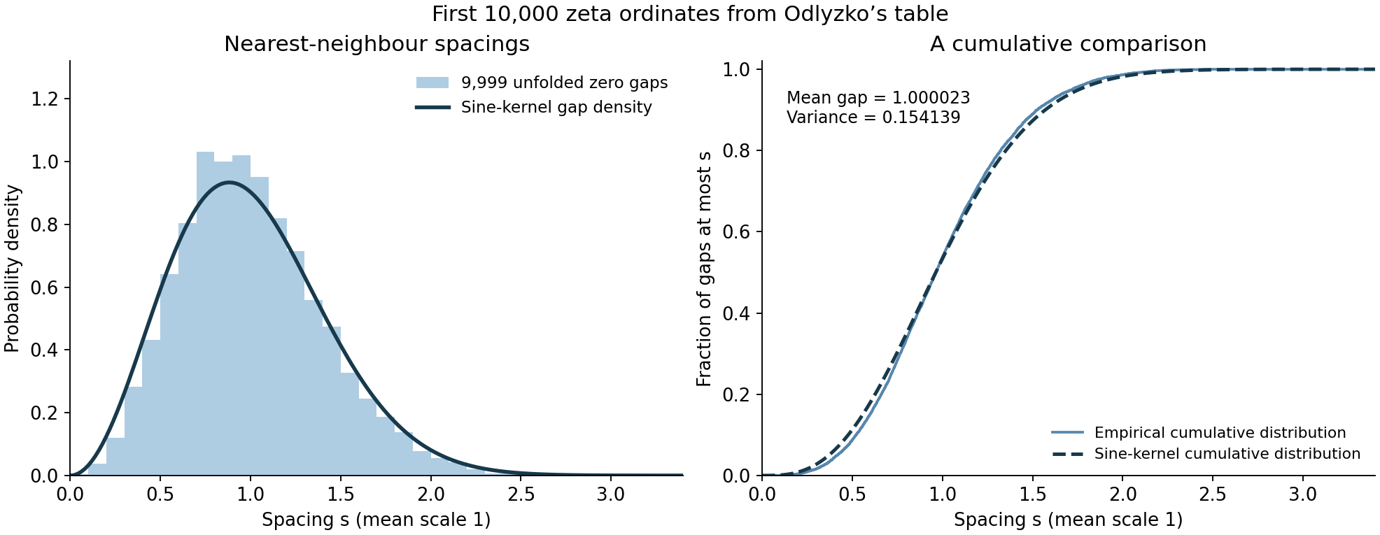
Figure 1. The first \(10,000\) ordinates in Odlyzko's numerical table produce \(9,999\) gaps. The left panel uses bins of width \(0.1\); the right panel compares cumulative distributions. The curve is \(E''(s)\) from (4.1), computed by Gauss–Legendre quadrature, rather than the two-dimensional Wigner approximation. An original reproducing script and vector image accompany the figure.
The mean gap is \(1.000023\), its population variance \(0.154139\), the smallest \(0.0420984\), and the largest \(2.483512\). About \(21.5722\%\) are below \(0.68\). These are descriptions of this finite sample. They neither prove the limiting gap distribution nor upgrade the preceding lesson's infinitely-often small-gap theorem to a numerical proportion theorem.
To evaluate the determinant, map \((0,s)\) to \((0,1)\). If \(u_i,w_i\) are Gauss–Legendre nodes and weights on that interval, the symmetric quadrature matrix is \[ D_{ij}(s)=\sqrt{w_iw_j}\,sK(s(u_i-u_j)). \] Let \(B=I-D\). Direct differentiation gives \[ D_{ij}'=\sqrt{w_iw_j}\cos(\pi s(u_i-u_j)),\qquad D_{ij}''=-\sqrt{w_iw_j}\,\pi(u_i-u_j)\sin(\pi s(u_i-u_j)). \] Differentiating \(\log\det B\) then gives the density estimate \[ (\det B)\left\{ [\operatorname{tr}(B^{-1}B')]^2 -\operatorname{tr}[(B^{-1}B')^2] +\operatorname{tr}(B^{-1}B'') \right\}. \tag{13.1} \] On \(0\leq s\leq3.4\) with grid step \(0.02\), changing from 64 to 96 nodes changed the computed density by at most \(5.9\times10^{-15}\). Its trapezoidal integral on that grid was \(0.9999977\). This is a floating-point convergence comparison, not a certified error interval. The primary table states absolute errors at most \(3\times10^{-9}\) for each ordinate; even that stated precision far exceeds what these plot bins need.
This low-zero plot is distinct from Odlyzko's experiments near the \(10^{20}\)-th zero. His 1992 revision of the large-height computation concerns that zero and 175 million neighbours; Katz–Sarnak's 1999 survey also displays the earlier 70-million-zero comparison. Those experiments are evidence at much higher heights. Finite computations and restricted-support theorems support the unitary prediction in complementary ways.
14. Exercises and solutions
1. The fourth-moment arithmetic factor. Prove \(a_2=\prod_p(1-p^{-2})=6/\pi^2\), and find \(a_2f_2\).
Solution. The generalized divisor coefficient is \(d_2(p^m)=m+1\). Starting with \(\sum x^m=(1-x)^{-1}\), apply \(x\,d/dx+1\) twice to obtain \(\sum(m+1)^2x^m=(1+x)/(1-x)^3\). Multiplication by \((1-x)^4\) leaves \(1-x^2\). Its product converges absolutely because \(\sum_pp^{-2}<\infty\), and the Euler product gives \(1/\zeta(2)=6/\pi^2\). Formula (7.4) gives \(f_2=0!1!/(2!3!)=1/12\), so the product is \(1/(2\pi^2)\).
2. Two integer constants. Compute \(g_3\) and \(g_4\) from the Barnes factor.
Solution. The recurrence \(G(n+1)=\Gamma(n)G(n)\), \(G(1)=1\), gives \(f_3=(0!1!2!)/(3!4!5!)=1/8640\) and \(f_4=(0!1!2!3!)/(4!5!6!7!)=1/870912000\). Thus \(g_3=9!/8640=42\) and \(g_4=16!/870912000=24024\). The factorial in \(g_k\) is \((k^2)!\), rather than \(k!\).
3. Fourier transform of the pair measure. Include the diagonal in transforming the pair density.
Solution. Direct integration shows \(K=\mathcal F^{-1}\mathbf1_{[-1/2,1/2]}\). The convolution of this indicator with itself is \((1-|\alpha|)_+\), so \(\widehat{K^2}\) is that triangle. These identities hold against every Schwartz test, by the bounded frequency intervals and Fubini's theorem. Fourier inversion gives \(\widehat1=\delta_0\) and \(\widehat{\delta_0}=1\). Therefore \(\mathcal F(\delta_0+1-K^2)=1+\delta_0-(1-|\alpha|)_+=\delta_0+\min(|\alpha|,1)\). Omitting the first delta changes the constant Fourier contribution.
4. The Barnes product. Prove the finite product for \(f_k\) directly from the recurrence.
Solution. Iteration gives \(G(k+1)=\prod_{j=0}^{k-1}j!\) and \(G(2k+1)=\prod_{j=0}^{2k-1}j!\). Cancel one copy of \(\prod_{j<k}j!\) in the quotient \(G(k+1)^2/G(2k+1)\). The denominator that remains is \(\prod_{j=k}^{2k-1}j!=\prod_{j=0}^{k-1}(j+k)!\). This proves \(f_k=\prod_{j=0}^{k-1}j!/(j+k)!\) for every integer \(k\geq1\).
5. The second matrix moment. Prove \(\mathbb E|\det(I-U)|^2=N+1\) using exterior powers.
Solution. Expand the determinant as \(\sum_{j=0}^N(-1)^j\chi_j(U)\), where \(\chi_j=\operatorname{tr}\Lambda^jU\). Each wedge representation is irreducible: its torus weights indexed by \(j\)-element subsets are distinct, and permutation matrices act transitively on their one-dimensional weight spaces, so its commuting operators are scalar. The representations are inequivalent because \(tI\) acts by the different powers \(t^j\). Haar averaging of matrix units, as in Section 5, makes the character inner products \(\int\chi_j\overline{\chi_\ell}=\delta_{j\ell}\). On integrating the expanded absolute square, exactly its \(N+1\) diagonal terms remain. This also covers \(N=1\): \(\mathbb E|1-e^{i\theta}|^2=2\).
15. Proof inputs and further reading
The results proved here are the distributional Fourier identity; the finite CUE correlations and their sine limit; the GUE bulk limit; the Fredholm gap law; all CUE characteristic-polynomial moments in their integrability range; the Barnes asymptotic and arithmetic factors; restricted zeta \(n\)-level and triple correlations; and the finite-field equidistribution argument and worked pencil family. Assertions labelled conjectures are left conjectural.
The second-moment proof in Section 8.1 uses the uniform Riemann–Siegel formula, Theorem 5.4 and Lemma 5.3, and the continuous gamma phase, Proposition 5.3. These are written programme proofs, including the integer-cutoff endpoints.
The compact-group measure and approximation inputs just used have the written proofs linked below. The other source and proof dependencies listed here remain separate obligations; a lesson title alone is not proof that its needed argument is available:
- Dirichlet series and Euler products, The Gamma function, The Riemann–von Mangoldt formula, The prime number theorem with its classical error term, and Mean values of Dirichlet polynomials and of zeta on the critical line in The Riemann zeta function, lessons 1, 3, 10, 12 and 16: absolute Euler products; Stirling and differentiated gamma estimates; the zero count and unit-interval bound; the prime number theorem for partial summation; the polarized mean-value inequality and the fourth-moment term (8.5). The second-moment formula (8.4) is proved in Section 8.1 above.
- The symmetric groups III: characters and symmetric functions, Theorem 3.1, and Corollary 4.1, equation (34): the labelled Frobenius characteristic and power-sum expansion in (9.3). Young tableaux and Young symmetrizers, Lemma 2.2, supplies the dominance-cancellation input to the labels; Proposition 4.2 and Theorem 4.3, supply cycle centralizers and classification. Characters and the orthogonality relations, Theorem 4.1 and Corollary 4.2, supply completeness and column orthogonality.
- Fourier analysis and class functions, Theorem 2.3, with Peter–Weyl, Theorem 4.1, supplies uniform approximation by characters on compact Hausdorff groups. The Weyl integration formula, Theorem 3.1, Corollary 4.4 and equation (4.6), supplies the normalized \(U(N)\) and \(USp(2g)\) measures and the general compact connected Lie-group formula. Its regular-cover and measurable change-of-variables proofs are included. The unitary Schur-character inputs are supplied by the next item. The orthogonal roots and normalized Weyl formula are supplied by the exact RT-CPT-07/08 routes in Section 10; its comparison (10.2a)–(10.2d) supplies positive spectral-angle folding and normalization. The compact-to-algebraic symplectic comparison (10.3d)–(10.3f) supplies the representation input there. These arguments retain the providers’ stated earlier foundations; measure and approximation alone do not establish them.
- Unitary groups: characters, dimensions and branching, Theorem 2.2 and equation (2.4): the full \(U(n)\) character classification, including negative integer weights, and Schur orthogonality used in (9.3). Its Theorem 5.1 supplies the additional tensor proof above. The orthogonal root systems have the exact RT-CPT-07 provider specified in Section 10, and their normalized spectral-density comparison is proved in (10.2a)–(10.2d). The algebraic symplectic characters used there are supplied by its rational highest-weight construction, not by the unitary calculation. No new clearance of all recursive provider foundations follows from these comparisons.
- the classical-root and normalizer calculation in RT-CPT-07 and Theorem 3.1 and equations (3.3)–(3.5) of the Weyl-integration lesson supply the orthogonal root factors, the even/odd normalizers and normalized Haar integration. Section 10’s comparison keeps the spectral versus conjugacy-class distinction, all ranks, labeling convention, determinant constants and compact-uniform kernel limit explicit; it does not replace the providers’ earlier foundations.
- Proposition 4.1 of the highest-weight lesson, Lemma 2.4 and its Lie-to-group argument, and Theorem 3.1, highest-weight uniqueness supply the compact symplectic lattice, cyclic highest line and uniqueness. Proposition 1.2 of the compact-representation lesson and Theorem 2.1, matrix-coefficient orthogonality supply complete reducibility and the matrix units. The comparison (10.3d)–(10.3f) then constructs the rational algebraic representation, proves absolute irreducibility after coefficient extension, and identifies pure Frobenius character values. Its inherited root and PBW foundations remain the exact providers specified in the highest-weight lesson; this is not a new certification of all their recursive dependencies.
- Poincaré duality for smooth varieties, Theorem 10.1, and the normalized trace, Theorem 2.1: finite-coefficient duality and its base-change normalization. The coefficient-limit proof (10.3a)–(10.3c) above supplies the Frobenius-equivariant lisse coinvariant formula with twist \((-d)\), using the ℓ-adic perfect-complex comparison, Theorem 6.1 and Theorem 7.2. Proper and smooth base change from the étale course, lessons 13 and 15, remain the inputs for the sheaves in the geometric family.
- The trace formula in all dimensions, Theorem 5.1, with Lemma 2.1: compact-support trace for characteristic-zero adic coefficients and its geometric-Frobenius comparison. The coefficient-limit proof is present; its finite-level curve trace and perfectness inputs remain distinct prerequisites. The current compact-support Theorem 12.3 and Corollary 12.4 give the general constructibility reduction and finiteness deduction, with their specified affine-line provider retained, not silently replaced by duality. Lefschetz pencils and vanishing cycles, Theorem 1.0, Propositions 1.1–1.2, Theorem G.1, Proposition 4.1 and Corollary 4.2, and Theorem 6.1 give the precise plane-pencil geometry, invariant comparison, conjugacy, irreducibility and openness used above. The direct curve Riemann hypothesis, Theorem 5.3, and Corollary 5.1 give weight-one purity and the zeta numerator. The Riemann hypothesis over finite fields, Theorem 1.1 is the broader smooth-projective result, preserved as a further route rather than needed for this curve example. These written arguments retain their exact local-comparison, cover-theoretic, smooth-base-change, duality and coherent-duality prerequisites. Linking their proofs does not certify every recursive foundation or extend the even-dimensional characteristic-two tame theorem.
- Weights, purity and semisimplicity over finite fields, Theorem D.3, equation (D.11): the written compact-support deduction bounds \(R^if_!\) by weight \(i\) for a weight-zero input. Its structure-morphism case is the precise estimate in (10.5). Appendices A–D retain the optimal curve estimate, ordinary cohomological comparisons and relative tame boundary compatibility with their full adic hypotheses. Those recursive foundations remain separate proof obligations; the higher-dimensional deduction is not an unwritten assignment, and its presence does not certify all of those foundations.
The primary works providing the comparisons are Montgomery, The pair correlation of zeros of the zeta function (1973), especially Dyson's observation; Keating–Snaith, Random matrix theory and \(\zeta(1/2+it)\) (2000), equations (15)–(16) for the matrix moment; and Conrey, Notes on \(L\)-functions and random matrix theory (2006), Sections 2–5. The determinant proof in Section 6 establishes the matrix formula.
For higher zeros, Rudnick–Sarnak, Zeros of principal \(L\)-functions and random matrix theory (1996), Theorems 1.1–1.2 and Sections 3–4, treat more general primitive automorphic \(L\)-functions as well as zeta. Hejhal's 1994 theorem on the triple correlation of zeta zeros precedes that general theorem; its hexagonal support and leading determinant are displayed in Conrey–Snaith, Triple correlation of the Riemann zeros (2008), introduction. Section 9 proves the zeta case used in this course; no assertion about general automorphic coefficients is used.
Katz–Sarnak, Zeroes of zeta functions and symmetry (1999), Sections 2–4, explains the distinction between bulk spacings and central family statistics. Bogomolny, Riemann zeta function and quantum chaos (2007), the spectral-statistics section, gives the time-reversal comparison. CFKRS, Integral moments of \(L\)-functions (2005), Conjecture 1.5.1 and Sections 2.1–2.2, supplies the conjectural recipe (12.1)–(12.2).