Complex manifolds and Kähler metrics

Draft — Self-checked by the writing AI. This chapter develops complex coordinates, adapted connections, Kähler metrics and potentials, projective and torus examples, and the octonionic six-sphere. Parts J–N prove the full smooth integrability theorem, including the Hilbert-space, Fourier, Sobolev and local elliptic arguments needed to construct smooth complex coordinates. They also prove the converse construction of complex charts and isothermal coordinates on every oriented metric surface.

Complex geometry connects two descriptions of a tangent vector: real coordinates and multiplication by $i$. We first establish the analytic test that relates them. We then examine the tangent-space splitting, its obstruction to closure under brackets, and the connections and metrics compatible with it.

All manifolds are finite dimensional, smooth, Hausdorff, second countable and without boundary. Complexification extends real tensors complex bilinearly; it does not change a real metric into a sesquilinear form. Our conventions are $\omega(X,Y)=g(JX,Y),\qquad N_J(X,Y)=[JX,JY]-J[JX,Y]-J[X,JY]-[X,Y].$ We use the proved calculus in Local tools, Lemma 0.3, smooth inverses in its Theorem 1.2, and the exterior derivative and bracket evaluation in Curvature and holonomy, Lemma A.2. Exact additional prerequisites are linked when used.

A. An analytic test for complex coordinates

For $z^j=x^j+iy^j$, put $\partial_j=\tfrac12(\partial_{x^j}-i\partial_{y^j}),\qquad \partial_{\bar j}=\tfrac12(\partial_{x^j}+i\partial_{y^j}).$ Here a holomorphic function means a function locally represented by a complex power series absolutely convergent on a neighbourhood. The next two proofs establish the equivalent smooth differential test, including the integral formula it needs. For the normalization of the planar integrals one may use the definition $\pi=2\int_{-1}^1(1+t^2)^{-1}\,dt$.

Lemma A.1 (a planar integral identity). Let $Q$ be an open rectangle with sides parallel to the coordinate axes, and let $f$ be smooth on a neighbourhood of its closure. Orient its boundary counterclockwise. For $z\in Q$, $f(z)=\frac1{2\pi i}\int_{\partial Q}\frac{f(\zeta)}{\zeta-z}\,d\zeta -\frac1\pi\int_Q\frac{\partial_{\bar\zeta}f(\zeta)}{\zeta-z}\,dA(\zeta). \tag{A.1}$ The last integral exists as an improper integral with the singular point removed.

Proof. We spell out the integration facts needed for this particular domain. For a continuous function on a rectangle, uniform continuity makes the oscillation on every sufficiently small rectangular cell uniformly small. Upper and lower rectangular sums differ by at most the total area times that oscillation. Their common limit defines the area integral. Comparing a product partition with the successive one-dimensional sums shows that either order of iterated integration has that same value. This proves the needed interchange directly from the one-dimensional integral in Local tools 0.3. It also proves the bound by area times the supremum and interchange with uniform limits.

The fundamental theorem of calculus on horizontal and vertical segments now gives, for a smooth complex-valued $G$, $\int_Q\partial_xG\,dA=\int_{\partial Q}G\,dy,\qquad \int_Q\partial_yG\,dA=-\int_{\partial Q}G\,dx.$ Consequently $\int_{\partial Q}G\,d\zeta=2i\int_Q\partial_{\bar\zeta}G\,dA$. The same formula holds for $Q$ with a smaller axis-parallel closed rectangle removed: subdivide along the four sides of the inner rectangle, apply the formula to the remaining rectangles, and cancel every interior edge with its oppositely oriented neighbour. The inner boundary has clockwise orientation in the resulting sum.

Remove the square $S_\epsilon=\{|\Re(\zeta-z)|<\epsilon,\ |\Im(\zeta-z)|<\epsilon\}$. Away from $z$, differentiating $1/(\zeta-z)$ gives zero for its $\bar\zeta$ derivative. Apply the preceding identity to $G=f(\zeta)/(\zeta-z)$. With both individual boundary curves oriented counterclockwise this gives $\int_{\partial Q}\frac{f(\zeta)}{\zeta-z}\,d\zeta -\int_{\partial S_\epsilon}\frac{f(\zeta)}{\zeta-z}\,d\zeta =2i\int_{Q\setminus\overline S_\epsilon} \frac{\partial_{\bar\zeta}f(\zeta)}{\zeta-z}\,dA. \tag{A.2}$ On a square ring $S_r\setminus\overline S_{r/2}$, the absolute value of the kernel is at most $2/r$, and its area is at most $4r^2$. Thus its absolute integral is at most $8r$. Summing the geometric sequence of rings bounds the integral over $S_\epsilon$ by $16\epsilon$. A bounded numerator therefore gives a Cauchy limit as the removed square shrinks, and the omitted integral tends to zero. This also proves absolute integrability.

For the inner contour, uniform continuity and its perimeter $8\epsilon$ show that replacing $f(\zeta)$ by $f(z)$ changes the integral by at most $8\sup_{S_\epsilon}|f-f(z)|$, which tends to zero. The integral of $d\zeta/(\zeta-z)$ around that square is $2\pi i$. For an explicit calculation, its right side contributes $\int_{-\epsilon}^{\epsilon}\frac{i\,dt}{\epsilon+it} =i\int_{-\epsilon}^{\epsilon}\frac{\epsilon\,dt}{\epsilon^2+t^2} =i\int_{-1}^{1}\frac{ds}{1+s^2}=i\pi/2.$ The real part is odd and integrates to zero; the remaining substitution is just $t=\epsilon s$. Multiplication by $i$ leaves $d\zeta/(\zeta-z)$ unchanged and yields the same value on the other sides. The definition of $\pi$ given above therefore evaluates the whole contour without a trigonometric integration formula. Taking the limit in (A.2) proves (A.1), including its sign. □

Theorem A.2 (smooth Cauchy–Riemann criterion). A smooth map $F:U\subset\mathbb C^n\to\mathbb C^m$ is holomorphic exactly when $dF_z(iv)=i\,dF_z(v)\quad\text{for every }z,v. \tag{A.3}$ For a scalar component $f$, this is equivalent to $\partial_{\bar j}f=0$ for every $j$. Holomorphic functions are smooth, and their complex partial derivatives are holomorphic.

Proof. For a real differential, its values on the real coordinate vectors determine it. Commutation with $i$ says $f_{y^j}=i f_{x^j}$, which is precisely $\partial_{\bar j}f=0$. This holds component by component for maps.

Suppose first that these equations hold. Around a point $a$, choose a product of closed squares $Q_j$ contained in $U$. Apply A.1 in each variable, with the others fixed. Every area term vanishes. Successive substitution gives $f(z)=\frac1{(2\pi i)^n} \int_{\partial Q_1}\cdots\int_{\partial Q_n} \frac{f(\zeta)}{\prod_{j=1}^n(\zeta_j-z_j)} \,d\zeta_n\cdots d\zeta_1. \tag{A.4}$ These are successive integrals on finitely many compact segments; no interchange involving a singular kernel is needed. Choose each square centred at $a_j$, with half-side $r_j>0$. For $|z_j-a_j|\leq q_jr_j$, $q_j<1$, expand $\frac1{\zeta_j-z_j} =\sum_{k=0}^{\infty} \frac{(z_j-a_j)^k}{(\zeta_j-a_j)^{k+1}}.$ The finite geometric identity shows that the remainder is bounded by $q_j^{K+1}/(r_j(1-q_j))$ after degree $K$, uniformly on the contour. Products of the series are uniformly absolutely convergent there: their absolute sums are bounded by $\prod_j(r_j(1-q_j))^{-1}$. The integral bound in Local tools 0.3 permits termwise integration. Thus (A.4) is a power series in $z-a$, with coefficient bound $|c_\alpha|\leq \sup_{\prod\partial Q_j}|f|\,(4/\pi)^n \prod_j r_j^{-\alpha_j}. \tag{A.5}$ The perimeter of $Q_j$ is $8r_j$, which gives the stated constant. Every formally differentiated series converges uniformly on a smaller polydisc: the extra factor is a polynomial in each $\alpha_j$, and $\sum_{k\geq0}k^d q^k$ converges for $q<1$. To see the latter without a series theorem, choose $q<s<1$; the ratio of successive terms of $k^d(q/s)^k$ is eventually smaller than a fixed number below one, so these terms are bounded, and comparison with $\sum s^k$ suffices.

Uniform convergence of a derivative series justifies differentiation: integrate that series on a real coordinate segment, use Local tools 0.3 to pass its partial sums through the integral, and recover the difference of the original series at the endpoints. Repeat for each derivative. Hence the power series gives smoothness and complex partial derivatives of the same kind.

Conversely, choose positive radii $R_j$ whose closed polydisc lies in a neighbourhood of absolute convergence. Convergence at the point with coordinates $a_j+R_j$ bounds each $|c_\alpha|\prod_jR_j^{\alpha_j}$ by the finite sum of their absolute values. This is a coefficient bound of the same form as (A.5). The preceding smaller-polydisc argument therefore gives termwise derivatives of every order. Each monomial has zero $\bar z^j$ derivative, so the sum does also. A complex partial derivative is again a convergent power series. The argument for a map is the scalar argument on each of its finitely many components. □

Corollary A.3 (complex charts and inverse maps). A holomorphic map with invertible complex differential has a holomorphic local inverse. A smooth manifold with charts into $\mathbb C^n$ whose transitions are holomorphic has a well-defined smooth field $J$ with $J^2=-I$, obtained by transporting multiplication by $i$. A smooth map between two such manifolds is holomorphic precisely when its tangent map intertwines their $J$'s.

Proof. An invertible complex-linear map is also invertible as a real map. The smooth inverse theorem Local tools 1.2 supplies a smooth local inverse $G$, whose derivative is $dG=(dF)^{-1}$. The inverse of a map commuting with $i$ also commutes with $i$, as follows by multiplying $dF\,i=i\,dF$ by its inverse on both sides. A.2 makes $G$ holomorphic.

On overlapping charts, A.2 says that the transition differential commutes with multiplication by $i$. Thus the two transported endomorphisms agree. Their squares are $-I$ and their coordinate coefficients are smooth. The same calculation for a map in a pair of charts converts the intrinsic intertwining equation exactly into (A.3). A.2 proves the last assertion. The chain rule also shows that compositions preserve the equation, hence are holomorphic. □

Lemma A.4 (a local right inverse with parameters). If $f(z,t)$ is smooth on $D\times V$, where $D\subset\mathbb C$ is a disc and $V$ is an open real parameter set, then on every smaller disc $D'$ with closure contained in $D$ there is a smooth $Tf$ satisfying $\partial_{\bar z}Tf=f$. The operator can be chosen linear and commuting with all derivatives in $t$.

Proof. Choose a smooth cutoff $\chi$ compactly supported in $D$, equal to one near $\overline{D'}$, using Local tools 3.1. Extend $F=\chi f$ by zero in its first variable and set $Tf(z,t)=\frac1\pi\int_{\mathbb C}\frac{F(z-w,t)}{w}\,dA(w) =-\frac1\pi\int_{\mathbb C}\frac{F(\zeta,t)}{\zeta-z}\,dA(\zeta). \tag{A.6}$ The equality follows from the translation and reversal $\zeta=z-w$; their real Jacobian has determinant one. It can also be obtained directly by translating the rectangular integral sums in A.1. Both integrals converge absolutely by the square-ring bound in A.1 and compact support.

On a compact set of $(z,t)$, the supports in the first integral lie in one bounded square. Every derivative of its numerator is uniformly bounded there. Difference quotients for a derivative of $F(z-w,t)$ converge uniformly to the corresponding derivative on that square, by the segment formula and uniform continuity. Multiplying the uniform error by the finite integral of $1/|w|$ proves passage of that derivative through the integral. Iteration proves smoothness of $Tf$, and proves commutation with all parameter derivatives.

In particular, differentiation in $\bar z$ using the first expression, followed by the same variable change, gives $\partial_{\bar z}Tf(z,t) =-\frac1\pi\int_{\mathbb C} \frac{\partial_{\bar\zeta}F(\zeta,t)}{\zeta-z}\,dA(\zeta) =F(z,t).$ For the last equality apply A.1 on a rectangle containing $z$ and the support of $F$ in its interior; the boundary integral is zero. On $D'$, $F=f$, as required. For complex parameters their real derivatives commute with $T$, so their Wirtinger derivatives do too. □

B. Splitting tangent vectors and measuring the obstruction

An almost complex structure is a smooth real endomorphism $J:TM\to TM$ satisfying $J^2=-I$. An integrable almost complex structure is one induced by complex charts as in A.3. We reserve this latter word for the existence of those charts.

Lemma B.1 (eigenspaces, covectors and bidegrees). An almost complex structure gives a smooth direct sum $TM\otimes_{\mathbb R}\mathbb C=E_+\oplus E_-, \qquad P_+=\tfrac12(I-iJ),\quad P_-=\tfrac12(I+iJ). \tag{B.1}$ Here $J$ acts by $i$ on $E_+$, by $-i$ on $E_-$, and conjugation exchanges the two. Both bundles have complex rank $n=\frac12\dim_{\mathbb R}M$. Their dual splitting yields spaces of forms $\Omega^{p,q}$. The map $J^*\alpha=\alpha\circ J$ has eigenvalue $i$ on covectors of type $(1,0)$, which annihilate $E_-$, and eigenvalue $-i$ on type $(0,1)$.

Proof. Multiplication using $J^2=-I$ gives $P_\pm^2=P_\pm$, $P_+P_-=0$, $P_++P_-=I$, and $JP_\pm=\pm iP_\pm$. Conjugation exchanges the projections because $J$ is real. Thus the two eigenspaces have equal dimension and sum to the whole complexification.

For completeness, a real vector space with $J^2=-I$ has a basis $v_1,Jv_1,\ldots,v_n,Jv_n$. A nonzero $v$ and $Jv$ are independent: a real relation $Jv=cv$ would imply $c^2=-1$. Having constructed some pairs, their span is $J$-invariant. Apply the same argument in the quotient by that span and lift a new vector to continue. This process terminates with even dimension. The vectors $v_j-iJv_j$ and their conjugates are bases of the two complex eigenspaces. Extend the $v_j$'s locally as smooth real vector fields. Their determinant stays nonzero near the initial point, so these formulas give smooth local frames of $E_\pm$.

A covector decomposes by precomposition with $P_+$ and $P_-$. The first component vanishes on $E_-$ and obeys $\alpha(JX)=i\alpha(X)$; the other has the opposite sign. Wedges of $p$ covectors of the first type and $q$ of the second type form a basis for the corresponding summand of degree $p+q$: take the duals of the local eigenbasis and the usual ordered wedge basis. This proves the direct bidegree decomposition and its smoothness. In a complex chart these bases are $dz^j,d\bar z^j$, dual to $\partial_j,\partial_{\bar j}$; direct evaluation gives all four pairings. □

Lemma B.2 (the tensor seen in brackets). The expression $N_J$ in the introduction is a smooth alternating real tensor. Its complexification satisfies, for sections $U,V$ of $E_+$ and $A,B$ of $E_-$, $N_J(U,V)=-4P_-[U,V],\quad N_J(A,B)=-4P_+[A,B],\quad N_J(U,A)=0. \tag{B.2}$ Consequently $N_J=0$ exactly when both eigenspace bundles are closed under Lie brackets. For real fields, $N_J(JX,Y)=N_J(X,JY)=-JN_J(X,Y),\qquad N_J(JX,JY)=-N_J(X,Y). \tag{B.3}$ An integrable structure has $N_J=0$. In real dimension two this tensor always vanishes.

Proof. The complexified bracket is complex bilinear over constants. Substitution of $JU=iU$, $JV=iV$ gives $N_J(U,V)=-2[U,V]-2iJ[U,V]=-4P_-[U,V].$ Using $-i$ instead gives the second formula; the two mixed terms cancel in the third. The bracket product rule $[fU,V]=f[U,V]-V(f)U$, proved in Principal bundles C.3, shows that $P_-[U,V]$ is linear over smooth functions in both $E_+$ arguments, since $P_-U=P_-V=0$. The same holds for $P_+[A,B]$. Mixed components vanish, and B.1 decomposes arbitrary fields into these components. Hence $N_J$ is tensorial. Skewness follows from the bracket, and its coordinate expression is smooth and real.

For two plus arguments the output in (B.2) is minus type; multiplying an input by $J$ therefore has the same effect as applying $-J$ to the output. The same observation with the signs reversed applies to two minus arguments. Mixed components vanish, so bilinear extension proves the first identities in (B.3). Applying one of them twice proves the last.

Formula (B.2) proves the bracket criterion. In a complex chart, $E_+$ is spanned by the commuting fields $\partial_j$. The bracket product rule shows that the bracket of arbitrary combinations of them is again in their span. Conjugation handles $E_-$, proving the integrable implication. In dimension two, each eigenspace has rank one. The bracket of $fU$ and $hU$ is $(fU(h)-hU(f))U$, hence stays in that rank-one bundle. The criterion proves the final assertion. This argument by itself does not construct complex charts on an arbitrary real surface. □

Theorem B.3 (exterior differentiation and the obstruction). For any almost complex structure the exterior derivative decomposes into bidegrees $\begin{gathered} d=\mu+\partial+\bar\partial+\bar\mu,\\ |\mu|=(2,-1),\qquad|\partial|=(1,0),\\ |\bar\partial|=(0,1),\qquad|\bar\mu|=(-1,2). \end{gathered} \tag{B.4}$ The following are equivalent: $N_J=0$; $d=\partial+\bar\partial$; and $\bar\partial^2 f=0$ for every smooth local complex-valued function. When they hold, on all forms, $\partial^2=0,\qquad\bar\partial^2=0,\qquad \partial\bar\partial+\bar\partial\partial=0. \tag{B.5}$

Proof. In a local eigen-coframe, every form is a sum of functions times wedges of one-forms of the two types. Differentiating a function adds either type. Differentiating a $(1,0)$-form gives a two-form, with possible types $(2,0),(1,1),(0,2)$; replacing that one-form inside a wedge therefore changes the type by $(1,0),(0,1),(-1,2)$. A $(0,1)$-factor gives $(2,-1),(1,0),(0,1)$. The exterior product rule proves that these are all the possible changes in any degree, giving (B.4) by projection. It also shows that each component has the corresponding graded product rule.

If $\alpha$ has type $(0,1)$, the exterior evaluation formula Curvature A.2, on $U,V\in E_+$, gives $(\mu\alpha)(U,V)=-\alpha([U,V]) =\tfrac14\alpha(N_J(U,V)). \tag{B.6}$ The derivative terms vanish since $\alpha(U)=\alpha(V)=0$ as functions. The conjugate formula describes $\bar\mu$ on $(1,0)$-forms. These two operators vanish on functions and on the other type of one-form. Since functions and the eigen-coframe generate the exterior algebra locally, their product rules show that $\mu=\bar\mu=0$ precisely when the right sides of (B.6) and its conjugate vanish. Covectors of each type separate vectors of that type. B.2 therefore proves the equivalence with $N_J=0$.

On $A,B\in E_-$, $\bar\partial f$ takes the values $Af,Bf$. A second exterior evaluation gives $\begin{aligned} (\bar\partial^2f)(A,B) &=A(Bf)-B(Af)-(P_-[A,B])f\\ &=(P_+[A,B])f =-\tfrac14\,df(N_J(A,B)). \end{aligned} \tag{B.7}$ If this vanishes for all local functions, take real coordinate functions whose differentials span the complexified cotangent space at a given point. Then $N_J(A,B)=0$ there. Conjugation and the mixed formula in B.2 give $N_J=0$. The converse follows from (B.7).

Finally $d^2=0$, including its coordinate proof from commuting mixed partials, is established in the exterior-calculus prerequisites of Curvature A.1–A.2. If $d=\partial+\bar\partial$, apply $d^2$ to a pure-type form. Its three output types are distinct. Their components are $\partial^2$, $\partial\bar\partial+\bar\partial\partial$, and $\bar\partial^2$, and each is zero. This proves (B.5). On a complex chart the definitions explicitly give $\partial=\sum_j dz^j\wedge\partial_j$ and $\bar\partial=\sum_j d\bar z^j\wedge\partial_{\bar j}$ on coefficient functions and hence on all forms. □

Corollary B.4 (real vectors and the wrong-type bracket). For smooth real vector fields $X,Y$, put $X^+=P_+X$, $Y^+=P_+Y$. Then $P_-[X^+,Y^+]=-\tfrac14P_-N_J(X,Y),\qquad N_J(X,Y)=-8\operatorname{Re}\big(P_-[X^+,Y^+]\big). \tag{B.8}$ For a $(0,1)$-form $\alpha$, $(d\alpha)^{2,0}(X^+,Y^+)=\tfrac14\alpha(N_J(X,Y)). \tag{B.9}$

Proof. The tensor identities of B.2 imply $\begin{aligned} N_J(P_+X,P_+Y) &=\tfrac14\big(N_J(X,Y)-iN_J(JX,Y)-iN_J(X,JY)-N_J(JX,JY)\big)\\ &=\tfrac12\big(N_J(X,Y)+iJN_J(X,Y)\big)=P_-N_J(X,Y). \end{aligned}$ The plus-plus bracket identity in B.2 says that the left side is $-4P_-[X^+,Y^+]$. This gives the first formula of (B.8). Since $N_J(X,Y)$ is real, the real part of its $P_-$ projection is half of it, proving the second formula with its factor $8$.

The two derivative terms in the exterior evaluation of $d\alpha(X^+,Y^+)$ vanish because $\alpha$ annihilates plus-type vectors. The remaining term is $-\alpha([X^+,Y^+])$. The minus projection is the only component that $\alpha$ detects. Substituting (B.8), and using $\alpha\circ P_-=\alpha$, proves (B.9). This also explains why the coefficient for the dual exterior calculation is $1/4$. □

C. A connection whose torsion is exactly the obstruction

A connection $D$ on $TM$ is adapted to $J$ when $D_X(JY)=J D_XY$. Equivalently, its complexification preserves each of the bundles in B.1. Its torsion is $T_D(X,Y)=D_XY-D_YX-[X,Y]$, with the tensoriality proved in Linear and affine connections D.1.

Theorem C.1 (an adapted connection with prescribed torsion). Every almost complex manifold has a real adapted connection with $T_D=\tfrac14N_J. \tag{C.1}$ It has a torsion-free adapted connection if and only if $N_J=0$.

Proof. A smooth positive metric exists by Principal bundles D.2; Riemannian connections A.1 supplies its torsion-free connection $\nabla^0$. The auxiliary metric need not be compatible with $J$. Complexify this connection. For $U,V\in E_+$, $A,B\in E_-$, define $\begin{aligned} D_UV&=P_+\nabla^0_UV,&D_AB&=P_-\nabla^0_AB,\\ D_AV&=P_+[A,V],&D_UB&=P_-[U,B]. \end{aligned} \tag{C.2}$ Extend by addition after decomposing each argument by B.1.

In the same-type cases, the connection axioms follow from those of $\nabla^0$, since projection fixes the second argument. In the mixed case, for example, $P_+[fA,V]=fP_+[A,V],\qquad P_+[A,fV]=A(f)V+fP_+[A,V].$ The term $-V(f)A$ in the first expression disappears under $P_+$. These are exactly linearity over functions in the first input and the Leibniz rule in the second. The other mixed case is identical with the signs interchanged. Summing all four components proves the connection axioms for arbitrary complex fields. Every operation is smooth and intrinsic. Conjugation exchanges the two same-type formulas and the two mixed formulas, so $D$ takes real fields to real fields. The output has the same type as its second argument; hence $D$ preserves $J$.

Since $\nabla^0$ is torsion-free, $T_D(U,V)=P_+[U,V]-[U,V]=-P_-[U,V]=\tfrac14N_J(U,V).$ The minus-type formula is the conjugate. For the mixed pair $A,V$, $T_D(A,V)=P_+[A,V]-P_-[V,A]-[A,V]=0.$ B.2 now proves (C.1) on every pair.

If $N_J=0$, this particular $D$ is torsion-free. Conversely, if an adapted connection is torsion-free and $U,V\in E_+$, then $[U,V]=D_UV-D_VU$ is in $E_+$. The conjugate assertion holds for $E_-$, so B.2 gives $N_J=0$. This proves both directions without invoking a theorem that constructs complex charts. □

Proposition C.2 (a metric connection preserving an arbitrary almost complex structure). Suppose $g$ is a positive real metric with $g(JX,JY)=g(X,Y)$, and let $\nabla$ be its Levi-Civita connection. Write $A_X=\nabla_XJ$. The formula $\widehat D_XY=\nabla_XY-\tfrac12JA_XY \tag{C.3}$ defines a real connection preserving both $g$ and $J$. Its torsion is $T_{\widehat D}(X,Y)=-\tfrac12J(A_XY-A_YX). \tag{C.4}$ Thus existence of a metric connection preserving $J$ requires no assumption that $N_J$ vanish.

Proof. The Levi-Civita connection exists by Riemannian connections A.1. The tensor derivative rules of Linear and affine connections C.1 make $A$ smooth and bilinear over functions in $X,Y$. Adding the displayed tensor to a connection preserves the connection axioms, as proved in Linear and affine connections A.3; all coefficients are real.

The relation $J^2=-I$, differentiated by $\nabla$, gives $A_XJ=-JA_X$. Compatibility of $g$ with $J$ also gives $g(JY,Z)=-g(Y,JZ)$, by replacing $Z$ with $-JZ$ in the compatibility equation. Differentiate this identity and use $\nabla g=0$. The vector-derivative terms cancel, leaving $g(A_XY,Z)=-g(Y,A_XZ)$. Thus both $J$ and $A_X$ are skew-adjoint. Consequently $(JA_X)^*=A_X^*J^*=A_XJ=-JA_X.$ The correction $Q_X=-JA_X/2$ is skew-adjoint. Expanding the derivative of $g(Y,Z)$ under $\widehat D=\nabla+Q$ now cancels its two correction terms, proving $\widehat Dg=0$.

Finally $JA_XJ=A_X$ and $JJA_X=-A_X$, so $[Q_X,J]=-\tfrac12(JA_XJ-JJA_X)=-A_X.$ The homomorphism derivative rule yields $(\widehat D_XJ)Y=A_XY+[Q_X,J]Y=0$. Since $\nabla$ is torsion-free, its torsion cancels in the definition for $\widehat D$, leaving $Q_XY-Q_YX$, which is (C.4). □

D. When a Hermitian metric is parallel

An almost Hermitian metric is a positive real metric $g$ with $g(JX,JY)=g(X,Y)$. On a complex manifold it is called Hermitian. A Hermitian metric is Kähler when its fundamental form $\omega(X,Y)=g(JX,Y)$ is closed.

Lemma D.1 (the metric and its real form). Every almost complex manifold has an almost Hermitian metric. For such a metric, $\omega$ is a real nondegenerate two-form of type $(1,1)$, and $\omega(X,JX)=g(X,X)>0$ for $X\ne0$. Conversely these properties of a real $(1,1)$-form recover a unique compatible metric $g(X,Y)=\omega(X,JY)$.

Proof. From any positive metric $b$ supplied by Principal bundles D.2, take $g(X,Y)=\frac12(b(X,Y)+b(JX,JY))$. It is smooth, positive, symmetric and unchanged when both arguments are multiplied by $J$. Substituting $-JY$ for $Y$ in this invariance shows $g(JX,Y)=-g(X,JY)$. Thus $\omega$ is skew. Its kernel is zero because $J$ and $g:TM\to T^*M$ are invertible. The displayed positivity follows from invariance.

Complexify. If $U,V\in E_+$, then invariance gives $g(U,V)=g(iU,iV)=-g(U,V)$, so $g(U,V)=0$. The same holds on $E_-$. Therefore $\omega$ vanishes on two equal-type arguments and has type $(1,1)$. The pairing of $E_+$ with $E_-$ is nondegenerate: a vector pairing to zero with the opposite type also pairs to zero with its own type, hence with the whole complexified tangent space, so is zero.

Conversely, the type $(1,1)$ condition is equivalent to $\omega(JX,JY)=\omega(X,Y)$: it holds on opposite-type pairs, and on equal-type pairs this equation forces their value to vanish. Skewness and this identity give $\omega(Y,JX)=-\omega(JX,Y)=\omega(X,JY).$ Thus $g(X,Y)=\omega(X,JY)$ is symmetric and positive by the assumed inequality, and is $J$-invariant. Finally $g(JX,Y)=\omega(JX,JY)=\omega(X,Y)$, proving that these two constructions are inverse. □

Theorem D.2 (the Kähler equivalences). Let $\nabla$ be the Levi-Civita connection of an almost Hermitian metric. Then $\nabla J=0\quad\Longleftrightarrow\quad N_J=0\ \text{and}\ d\omega=0. \tag{D.1}$ On a complex manifold this is equivalent to the metric being Kähler. It is also equivalent, there, to the existence of a torsion-free connection preserving both $g$ and $J$; that connection is uniquely $\nabla$.

Proof. If $\nabla J=0$, it preserves both eigenspace bundles. Its zero torsion and C.1's last argument give $N_J=0$. The tensor derivative rule Linear and affine connections C.1 gives $\nabla\omega=0$, since $\nabla g=0$. For a two-form and a torsion-free connection, direct expansion of the exterior evaluation formula gives $d\omega(X,Y,Z) =(\nabla_X\omega)(Y,Z)+(\nabla_Y\omega)(Z,X)+(\nabla_Z\omega)(X,Y). \tag{D.2}$ Indeed expand each covariant derivative into the derivative of the pairing minus its two vector-derivative terms; combine the latter in pairs using $\nabla_XY-\nabla_YX=[X,Y]$. The result is the alternating derivative-and-bracket formula in Curvature A.2. Thus $d\omega=0$.

Conversely suppose $N_J=0$ and $d\omega=0$. The two eigenspaces are involutive by B.2. To show that $\nabla_XV$ has plus type for $V\in E_+$, it suffices by the nondegenerate opposite-type pairing in D.1 to prove $g(\nabla_XV,W)=0$ for every $W\in E_+$. It is enough to treat $X$ of each pure type.

For $X=U\in E_+$, the full Koszul formula Riemannian connections A.1 has three derivatives of identically zero same-type pairings. Its three bracket terms also pair two plus vectors, because the brackets are plus type. It gives $2g(\nabla_UV,W)=0$.

For $X=A\in E_-$, the same formula becomes $\begin{aligned} 2g(\nabla_AV,W) ={}&Vg(W,A)-Wg(A,V)-g(A,[V,W])\\ &-g(V,[A,W])+g(W,[A,V]). \end{aligned} \tag{D.3}$ Evaluate $d\omega$ on $A,V,W$. In D.1's notation, $\omega(A,W)=-ig(A,W)$, while $\omega(B,W)=-ig(B,W)$ for any complex vector $B$, since only its minus component pairs with $W$. Also $[V,W]$ is plus type, so $\omega([V,W],A)=ig([V,W],A)$. The exterior evaluation formula therefore gives $\begin{aligned} d\omega(A,V,W) =i\bigl(&Vg(A,W)-Wg(A,V)-g([V,W],A)\\ &+g([A,V],W)-g([A,W],V)\bigr) =2i\,g(\nabla_AV,W). \end{aligned} \tag{D.4}$ Closedness makes this zero. We have proved preservation of $E_+$; conjugation proves preservation of $E_-$. Hence $\nabla J=0$.

On a complex manifold B.2 already gives $N_J=0$, so (D.1) is exactly the equivalence with closedness in the Kähler definition. A torsion-free metric connection is uniquely Levi-Civita by Riemannian A.1. It additionally preserves $J$ exactly when the conditions just proved hold. This proves the last assertion. □

Proposition D.3 (the coordinate coefficients). In a complex chart, write $h_{j\bar k}=2g(\partial_j,\partial_{\bar k}),\qquad \omega=\frac i2\sum_{j,k}h_{j\bar k}\,dz^j\wedge d\bar z^k. \tag{D.5}$ The matrix $h$ is Hermitian and positive in the sense that $\sum h_{j\bar k}v^j\bar v^k>0$ for $v\ne0$. The metric is Kähler precisely when $\partial_\ell h_{j\bar k}=\partial_jh_{\ell\bar k} \quad\text{for every }j,k,\ell. \tag{D.6}$ In that case its Levi-Civita coefficients obey $\nabla_{\partial_j}\partial_{\bar k} =\nabla_{\partial_{\bar k}}\partial_j=0,\qquad \nabla_{\partial_j}\partial_k =\sum_a\Gamma^a_{jk}\partial_a,\qquad \sum_a\Gamma^a_{jk}h_{a\bar\ell} =\partial_jh_{k\bar\ell}. \tag{D.7}$ The other coefficients are complex conjugates, and $\Gamma^a_{jk}=\Gamma^a_{kj}$.

Proof. Reality and symmetry of $g$ give $h_{j\bar k}=\overline{h_{k\bar j}}$. A real tangent vector with complex coordinate velocity $v$ is $\sum_j(v^j\partial_j+\bar v^j\partial_{\bar j})$; D.1 makes its squared norm $\sum h_{j\bar k}v^j\bar v^k$. This proves positivity. Evaluate $\omega$ on the coordinate eigenbasis, using $J\partial_j=i\partial_j$, to obtain (D.5), with the factor $1/2$ fixed by the definition of $h$.

More explicitly, the complex bilinear extension of the metric and its value on real vectors are $\begin{aligned} g_{\mathbb C}&=\frac12\sum_{j,k}h_{j\bar k} (dz^j\otimes d\bar z^k+d\bar z^k\otimes dz^j),\\ g(X,Y)&=\operatorname{Re}\sum_{j,k}h_{j\bar k} dz^j(X)\overline{dz^k(Y)}\qquad(X,Y\text{ real}). \end{aligned}$ The first formula agrees with $g$ on every pair of coordinate eigenvectors: equal-type pairs give zero and opposite-type pairs give $h_{j\bar k}/2$. Bilinearity therefore proves it on all vectors. On real vectors its two summands are conjugate after interchanging $j,k$ and using the Hermitian symmetry of $h$, proving the second formula. In particular $h=I$ gives $g=\sum_j((dx^j)^2+(dy^j)^2)$ and $\omega=\sum_j dx^j\wedge dy^j$, since $dz^j=dx^j+i\,dy^j$.

B.3's coordinate formula for $d$ shows that the $(2,1)$-coefficients of $d\omega$ are $i/2$ times the differences in (D.6). Its $(1,2)$ component is the complex conjugate, and no other type occurs. Thus closedness is equivalent to (D.6).

For a Kähler metric, D.2 says $\nabla$ preserves type. Torsion-freeness and commutation of the coordinate fields give $\nabla_{\partial_j}\partial_{\bar k}=\nabla_{\partial_{\bar k}}\partial_j$. The left side is minus type and the right side plus type. Their equality forces both to vanish. Metric compatibility then gives $\partial_j g(\partial_k,\partial_{\bar\ell}) =g(\nabla_{\partial_j}\partial_k,\partial_{\bar\ell}),$ which after multiplication by two is the last formula of (D.7). The matrix is invertible by its positivity, so these equations determine every coefficient. Zero torsion gives symmetry in $j,k$, and the real connection gives the conjugate formulas. □

Example D.4 (closedness alone does not suffice). There is a smooth almost Hermitian structure on $\mathbb R^4$ whose fundamental form is closed but whose Nijenhuis tensor is nowhere zero. On a Riemann surface, by contrast, every Hermitian metric is Kähler.

Proof. The real exponential, its positivity, its derivative and its addition law are proved in Local tools 0.5. With coordinates $x,y,u,v$, use the global frame $e_1=\partial_x,\quad e_2=\partial_y,\quad e_3=e^x\partial_u,\quad e_4=e^{-x}\partial_v.$ Define $Je_1=e_2,\ Je_2=-e_1,\ Je_3=e_4,\ Je_4=-e_3$, and make this frame orthonormal. Then $g=dx^2+dy^2+e^{-2x}du^2+e^{2x}dv^2,\qquad \omega=dx\wedge dy+du\wedge dv. \tag{D.8}$ The dual frame is $dx,dy,e^{-x}du,e^x dv$, which verifies both formulas and positive compatibility directly. The coefficients of $\omega$ are constant, hence $d\omega=0$. The only brackets needed are $[e_1,e_3]=e_3,\ [e_1,e_4]=-e_4,\ [e_2,e_3]=[e_2,e_4]=0$. Substitution into the definition gives $N_J(e_1,e_3)=0-0-J(-e_4)-e_3=-2e_3,$ which is nonzero everywhere. B.2 rules out complex charts inducing this $J$, and D.2 rules out its parallelism.

A Riemann surface already has complex charts and real dimension two. Its fundamental form is a two-form, whose exterior derivative is a three-form on a two-dimensional tangent space and therefore zero. Its Hermitian metric is Kähler by definition, and D.2 makes $J$ parallel. This assertion assumes the complex atlas. The converse construction of charts on every oriented metric surface is proved in N.2. □

Proposition D.5 (the full tensor identity behind the Kähler equivalence). On an almost Hermitian manifold with Levi-Civita connection $\nabla$, $2g((\nabla_XJ)Y,Z) =d\omega(X,Y,Z)-d\omega(X,JY,JZ)+g(N_J(Y,Z),JX). \tag{D.9}$ This identity holds without assuming integrability or closedness.

Proof. Set $A_XY=(\nabla_XJ)Y$ and $a(X,Y,Z)=g(A_XY,Z)$. The skew-adjointness and anticommutation calculations in C.2 give $\begin{aligned} a(X,Y,Z)&=-a(X,Z,Y),\\ a(X,JY,Z)&=a(X,Y,JZ),\\ a(X,JY,JZ)&=-a(X,Y,Z). \end{aligned} \tag{D.10}$ The tensor product rule, $\nabla g=0$, and the definition of $\omega$ give $(\nabla_X\omega)(Y,Z)=a(X,Y,Z)$. Alternating as in (D.2) therefore gives $d\omega(X,Y,Z)=a(X,Y,Z)+a(Y,Z,X)+a(Z,X,Y). \tag{D.11}$

We compute the other term directly from the definition of $N_J$, replacing every bracket by the difference of covariant derivatives. For the inputs $Y,Z$, the four bracket terms expand respectively to $\begin{aligned} {}[JY,JZ]&=A_{JY}Z-A_{JZ}Y+J\nabla_{JY}Z-J\nabla_{JZ}Y,\\ -J[JY,Z]&=-J\nabla_{JY}Z+JA_ZY-\nabla_ZY,\\ -J[Y,JZ]&=-JA_YZ+\nabla_YZ+J\nabla_{JZ}Y,\\ -[Y,Z]&=-\nabla_YZ+\nabla_ZY. \end{aligned}$ Thus $N_J(Y,Z)=A_{JY}Z-A_{JZ}Y+JA_ZY-JA_YZ$. Pairing with $JX$ and using (D.10) and the metric invariance under $J$ yields $\begin{aligned} g(N_J(Y,Z),JX) ={}&a(JY,JZ,X)-a(JZ,JY,X)\\ &-a(Z,X,Y)-a(Y,Z,X). \end{aligned} \tag{D.12}$ Meanwhile (D.11) and (D.10), evaluated on $X,JY,JZ$, yield $d\omega(X,JY,JZ) =-a(X,Y,Z)+a(JY,JZ,X)-a(JZ,JY,X).$ Subtract this last equality from (D.11) and add (D.12). Every term except $2a(X,Y,Z)$ cancels, proving (D.9). □

E. Constructing local potentials

This part starts on a complex manifold, where B.3 gives $\partial^2=\bar\partial^2=0$ and $\partial\bar\partial=-\bar\partial\partial$. A smooth real function $\phi$ is strictly plurisubharmonic when its matrix $(\partial_j\partial_{\bar k}\phi)$ is positive definite at every point of each complex chart.

Lemma E.1 (a local primitive for a closed $(0,1)$-form). If $\beta=\sum_{j=1}^n b_j\,d\bar z^j$ is smooth and $\bar\partial\beta=0$, then in a neighbourhood of each point there is a smooth complex function $f$ with $\beta=\bar\partial f$.

Proof. Work in a polydisc around the point. The coefficient condition is $\partial_{\bar j}b_k=\partial_{\bar k}b_j$. Apply the operator in A.4 to $b_1$ in its first coordinate, leaving the others as parameters. On a smaller first-coordinate disc set $f_1=T_1b_1$ and replace $\beta$ by $\beta-\bar\partial f_1$. The first coefficient becomes zero. The remaining form is still closed by B.3. Its coefficient equations now say that all remaining coefficients have zero $\bar z^1$ derivative.

Inductively suppose the first $r-1$ coefficients have been made zero on a product neighbourhood. The remaining coefficients have zero $\bar z^j$ derivative for $j<r$, by closedness. Apply A.4 in the $r$-th coordinate to its $r$-th coefficient, with a cutoff depending only on that coordinate. Its commutation with all other derivatives implies $\partial_{\bar j}f_r=0$ for $j<r$. Subtracting $\bar\partial f_r$ therefore leaves the first $r-1$ coefficients zero and makes the $r$-th zero. Closedness is preserved. After $n$ steps, all coefficients vanish on the final product neighbourhood. The finite sum $f=f_1+\cdots+f_n$, restricted there, is smooth and has the required derivative. □

Lemma E.2 (a real primitive on a coordinate ball). Every smooth closed real two-form on a ball centred at zero in $\mathbb R^m$ is $d\alpha$ for a smooth real one-form $\alpha$ on that ball.

Proof. Write $\omega=\frac12\sum_{i,j}\omega_{ij}(x)\,dx^i\wedge dx^j$, with $\omega_{ij}=-\omega_{ji}$, and set $\alpha_j(x)=\sum_i x^i\int_0^1 t\,\omega_{ij}(tx)\,dt, \qquad \alpha=\sum_j\alpha_j\,dx^j. \tag{E.1}$ The segment stays in the ball. The integrands and all their derivatives are continuous uniformly on compact subsets times $[0,1]$; the segment estimate of Local tools 0.3 permits differentiation under the integral, proving smoothness. The coefficients are real.

Closedness says $\partial_k\omega_{ij}-\partial_j\omega_{ik}=\partial_i\omega_{kj}$. Differentiate (E.1) in coordinates and subtract: $\begin{aligned} \partial_k\alpha_j-\partial_j\alpha_k &=\int_0^1\left(2t\,\omega_{kj}(tx) +t^2\sum_i x^i\partial_i\omega_{kj}(tx)\right)\,dt\\ &=\int_0^1\frac d{dt}\bigl(t^2\omega_{kj}(tx)\bigr)\,dt =\omega_{kj}(x). \end{aligned}$ The endpoint at zero vanishes because the coefficient is bounded there. These are exactly the coefficients of $d\alpha=\omega$. □

Theorem E.3 (real Kähler potentials and their ambiguity). Every smooth closed real $(1,1)$-form is locally $\omega=\frac i2\,\partial\bar\partial\phi \tag{E.2}$ for a smooth real function $\phi$. It is positive, meaning $\omega(X,JX)>0$ for nonzero real $X$, exactly when $\phi$ is strictly plurisubharmonic. Two real potentials for the same form differ, locally, by the real part of a holomorphic function; adding such a real part does not change the form.

Proof. Choose a complex coordinate ball. E.2 gives a real one-form $\alpha$ with $d\alpha=\omega$. Decompose it as $\alpha^{1,0}+\alpha^{0,1}$. Since $\omega$ has no $(0,2)$-part, $\bar\partial\alpha^{0,1}=0$. E.1 provides $f$ on a smaller neighbourhood such that $\alpha^{0,1}=\bar\partial f$. Reality gives $\alpha^{1,0}=\partial\bar f$. Therefore $\omega=\partial\bar\partial f+\bar\partial\partial\bar f =\partial\bar\partial(f-\bar f) =2i\,\partial\bar\partial\Im f.$ Taking $\phi=4\Im f$ gives (E.2) with the stated normalization.

In coordinates the coefficients of the resulting form are $(i/2)\partial_j\partial_{\bar k}\phi$. Reality of $\phi$ and equality of mixed real partials make this matrix Hermitian. Evaluation as in D.3 shows $\omega(X,JX)=\sum_{j,k}(\partial_j\partial_{\bar k}\phi)v^j\bar v^k$. This proves the positivity assertion and its coordinate independence: the left side is an intrinsic positive form.

Let $u$ be the difference of two real potentials. Then $\partial_{\bar k}(\partial_j u)=0$ for every $j,k$. By A.2, each $a_j=\partial_j u$ is holomorphic. Equality of mixed derivatives gives $\partial_k a_j=\partial_j a_k$. On a smaller coordinate ball centred at zero define $H(z)=2\sum_j z^j\int_0^1 a_j(tz)\,dt. \tag{E.3}$ Differentiation under the integral is justified by uniform smooth derivative bounds on compact subsets, as in E.2. Every $\bar z$ derivative is zero; A.2 makes $H$ holomorphic. Its $z^k$ derivative is $\begin{aligned} \partial_k H &=2\int_0^1\left(a_k(tz)+t\sum_jz^j\partial_k a_j(tz)\right)\,dt\\ &=2\int_0^1\frac d{dt}\bigl(t a_k(tz)\bigr)\,dt =2a_k(z). \end{aligned}$ Because $H$ is holomorphic, $\partial\Re H=\frac12\partial H=\partial u$; conjugation gives the same equality for $\bar\partial$. Thus every real partial derivative of $u-\Re H$ is zero. Integrating along segments by Local tools 0.3 shows it is constant on that ball. Add this real constant to $H$ to obtain $u=\Re H$. Conversely, if $u=\Re H$ with $H$ holomorphic, its mixed $z,\bar z$ derivatives vanish, so $\partial\bar\partial u=0$, proving the last assertion. □

Proposition E.4 (why a positive potential cannot be global on a compact manifold). A nonempty compact complex manifold of positive complex dimension has no smooth globally defined strictly plurisubharmonic function. In particular a Kähler form on it cannot have a globally defined real potential of the form in E.3.

Proof. A continuous real function $\phi$ on a compact space attains a maximum. Indeed its image is compact: an open cover pulls back to a cover of the domain and has a finite subcover. A compact subset of $\mathbb R$ is bounded by the cover $(-k,k)$, and contains its supremum because otherwise the complements of decreasing closed intervals about that supremum would cover it without a finite subcover. These statements also follow from Local tools 0.1.

Choose a maximum point and a complex chart about it. For every real coordinate direction, restriction to a short line segment has a maximum at zero. If its second derivative at zero were positive, continuity would make the second derivative positive on a smaller segment; the fundamental theorem of calculus applied twice, and the zero first derivative at a maximum, would make its value larger on that segment away from zero. Thus both $\phi_{x^jx^j}$ and $\phi_{y^jy^j}$ are nonpositive at the maximum. The definition of the Wirtinger derivatives gives $\partial_j\partial_{\bar j}\phi =\tfrac14(\phi_{x^jx^j}+\phi_{y^jy^j})\leq0.$ There is at least one such index because the complex dimension is positive. A positive definite complex Hessian has positive value on that coordinate vector, a contradiction. If a global potential for a Kähler form existed, E.3 would make its complex Hessian positive everywhere, giving the forbidden function. □

F. Complex frames, unitary frames and orientation

Proposition F.1 (the real bundle behind a complex structure). An almost complex structure on a real bundle of rank $2n$ is equivalent to a reduction of its frame bundle to $\mathrm{GL}(n,\mathbb C)$. It determines an orientation. A compatible positive metric is equivalent to a further reduction to $\mathrm U(n)$. On each fibre the associated Hermitian inner product, linear in its first argument, is $H(X,Y)=g(X,Y)-i\omega(X,Y). \tag{F.1}$ For a real vector $X$ and $Z=P_+X$, the complex bilinear extension of $g$ instead satisfies $g_{\mathbb C}(Z,Z)=0,\qquad g_{\mathbb C}(Z,\bar Z)=\tfrac12g(X,X). \tag{F.2}$

Proof. Define $(a+ib)X=aX+bJX$. Addition and distributivity follow from real linearity. Multiplication of two such operators uses $J^2=-I$ and gives $(aI+bJ)(cI+dJ)=(ac-bd)I+(ad+bc)J$, so this is a complex vector-space structure. Conversely multiplication by $i$ in any complex vector space is a real operator squaring to $-I$. A real map is complex linear precisely when it intertwines these operators.

The real paired bases and smooth local frames in B.1 show that the frames intertwining the standard $J_0$ with $J$ form, in each such local trivialization, exactly $U\times\mathrm{GL}(n,\mathbb C)$. This is an embedded principal subbundle: in real matrices the commutation equation $AJ_0=J_0A$ defines a linear subspace, and invertibility is open in that subspace. Its transition functions are smooth complex matrices, by the frame-coordinate theorem Principal bundles C.1–C.2. Conversely a frame reduction defines $J=uJ_0u^{-1}$; right multiplication of $u$ by a matrix commuting with $J_0$ leaves this expression unchanged. In its local sections it is smooth. These two constructions are inverse.

If $A=B+iC$ is complex invertible, its real matrix on paired coordinates is $A_{\mathbb R}=\begin{pmatrix}B&-C\\ C&B\end{pmatrix}.$ The permutation and multilinearity proof of the determinant identities in DG-CHAR-06 L.1 applies over $\mathbb C$ as well as $\mathbb R$: each sum, product and alternating cancellation is a field identity. After complexification, the invertible linear change $(x,y)\mapsto(x+iy,x-iy)$ changes this operator to $\operatorname{diag}(A,\bar A)$. Determinants of similar matrices agree by multiplicativity, and the determinant polynomial commutes with complex conjugation. Hence $\det_{\mathbb R}A_{\mathbb R} =\det_{\mathbb C}A\,\overline{\det_{\mathbb C}A} =|\det_{\mathbb C}A|^2>0. \tag{F.3}$ The real determinant has the same value when its real entries are regarded as complex entries, by the same permutation formula. Thus all complex paired frames induce the same real orientation.

D.1 gives $g(JX,Y)=\omega(X,Y)$ and $\omega(JX,Y)=-g(X,Y)$. Substituting in (F.1) yields $H(JX,Y)=iH(X,Y)$. Skewness of $\omega$ and symmetry of $g$ yield $H(Y,X)=\overline{H(X,Y)}$, and therefore conjugate linearity in the second argument. Positivity is $H(X,X)=g(X,X)>0$ for $X\ne0$.

Starting from a smooth complex frame $v_1,\ldots,v_n$, successively set $w_j=v_j-\sum_{k<j}H(v_j,e_k)e_k,\qquad e_j=w_j/\sqrt{H(w_j,w_j)}. \tag{F.4}$ Induction shows $H(w_j,e_k)=0$ for $k<j$, and the first $j-1$ vectors span the same complex space as the preceding $v_k$'s. Thus $w_j\ne0$ and its squared norm is positive. The positive square root is smooth by Principal bundles D.2, so these are smooth unitary frames. Any two differ by a unitary matrix, and conversely such a matrix preserves $H$. The equations $A^*A=I$ define an embedded subgroup in complex matrices: the derivative is $A^*B+B^*A$, which maps $B=AS/2$ to any prescribed Hermitian $S$ when $A^*A=I$; the smooth submersion theorem Local tools 1.3 applies. In each unitary frame chart the selected frames form $U\times\mathrm U(n)$, establishing the reduction.

A unitary reduction conversely transfers the standard Hermitian form to the fibres, independently of the chosen frame. Its real part gives the compatible positive $g$, and these constructions are inverse. In real matrices, being unitary is exactly being orthogonal and commuting with $J_0$; (F.3) shows these matrices lie in $\mathrm{SO}(2n)$.

Finally $Z=(X-iJX)/2$. Expand both bilinear pairings in (F.2), use $g(X,JX)=0$ and $g(JX,JX)=g(X,X)$, and obtain respectively zero and $g(X,X)/2$. This explicitly distinguishes the two uses of a complex-valued metric. Rank zero gives the trivial statements on a zero-dimensional fibre. □

Proposition F.2 (adapted transport and the full holonomy group). A real connection $D$ on an almost complex tangent bundle satisfies $DJ=0$ exactly when all its parallel maps intertwine the endpoint complex structures. These are precisely the connections on the complex frame reduction. If in addition $Dg=0$, transport preserves the compatible Hermitian form and restricts to the unitary frame reduction. In particular the full Levi-Civita holonomy group of a Kähler metric is a subgroup of $\mathrm U(n)$ in a unitary frame, with no assumption on the fundamental group.

Proof. Linear and affine connections A.2 provides transport on every finite piecewise smooth path and a parallel frame along each smooth piece. Linear and affine connections C.1 gives $D_t(JV)=(D_{\dot\gamma}J)V+JD_tV.$ If $DJ=0$ and $V$ is parallel, then $JV$ is parallel with the corresponding initial value. Uniqueness of parallel fields proves intertwining. Conversely suppose every parallel map intertwines $J$. For any tangent vector $X$ at a point, choose a smooth coordinate path whose initial velocity is $X$. Transport any initial vector $v$ along it. The hypothesis makes both $V$ and $JV$ parallel; the displayed rule at the initial point gives $(D_XJ)v=0$. Varying $X,v$ proves $DJ=0$.

In a complex frame from F.1, the operator $J$ is the constant matrix $J_0$. Writing $D=d+A$, the equation $DJ=0$ is $[A,J_0]=0$. Its entries are therefore complex-linear matrices. The frame formula of Linear and affine connections A.2, $\omega_{(x,h)}(X,\dot h)=h^{-1}A(X)h+h^{-1}\dot h,$ then restricts to a principal connection on the complex frame reduction: both terms are complex-linear, it reproduces the vertical generator, and right translation conjugates the value, exactly as in that theorem. Conversely a connection on the complex frames gives these complex-linear local matrices, hence commutes with $J_0$ and induces $DJ=0$.

If also $Dg=0$, the tensor product rule gives $\frac d{dt}g(V,W)=g(D_tV,W)+g(V,D_tW)=0$ for parallel fields. The fundamental theorem of calculus makes their pairing constant along each piece, and continuity gives the same assertion across the finitely many junctions. Since $\omega(V,W)=g(JV,W)$, both $\omega$ and $H=g-i\omega$ are preserved as well. Equivalently, in a unitary frame the matrix $A$ satisfies $A^*+A=0$: differentiate the constant pairings of its frame vectors and use metric compatibility. The preceding principal form consequently restricts to the unitary reduction. To check tangency directly, a horizontal frame matrix obeys $h'=-A(\dot\gamma)h$, so $(h^*h)'=-h^*(A^*+A)h=0.$ A frame initially unitary therefore stays unitary. The vertical space of the unitary group consists of the same skew-Hermitian matrices, by differentiation of $h^*h=I$, so the restriction has the required horizontal and vertical splitting.

For a Kähler metric, D.2 proves $\nabla J=0$, and Levi-Civita is metric compatible. Transport around every based loop therefore preserves $H$ on that tangent space. By definition the full holonomy group consists of all these loop transports; each is represented by a unitary matrix in the chosen unitary frame. The argument used every loop, rather than only contractible loops, which proves the stated full-group assertion. □

G. Projective space with its exact metric scale

Theorem G.1 (the projective potential and its eigenvalues). For $n\geq1$, complex projective space has compatible local potentials $\phi(z)=\log(1+|z|^2)$ and Kähler form $\omega_{\mathrm{FS}}=(i/2)\partial\bar\partial\phi$. Put $S=1+|z|^2$. Then $\begin{aligned} h_{j\bar k}&=\frac{S\delta_{jk}-\bar z^j z^k}{S^2},\\ g_z(v,v)&=\frac{S|v|^2-|z^*v|^2}{S^2},\qquad \det(h_{j\bar k})=S^{-(n+1)} . \end{aligned} \tag{G.1}$ At zero the metric is Euclidean. At nonzero $z$, its eigenvalue relative to the Euclidean metric is $S^{-2}$ on the complex line $\mathbb Cz$ and $S^{-1}$ on that line's Hermitian orthogonal complement. Each complex eigendirection accounts for two real directions. The global metric is complete.

Proof. The manifold, its quotient topology, compactness, smooth graph charts and holomorphic transitions are fully constructed in Hermitian symmetric spaces L.1, with $p=1,q=n$. Thus its points are complex lines $[Z_0:\cdots:Z_n]$, and on $Z_a\ne0$ the ratios $Z_j/Z_a$, $j\ne a$, are complex coordinates. We compute the metric in these actual charts.

For the real function $\log S$, differentiation gives $\partial_j\log S=\bar z^j/S$. A further $\bar z^k$ derivative gives the first formula in (G.1). D.3 gives the second by evaluation on a real vector of complex velocity $v$. At $z\ne0$, write $v=az+w$, where $a=(z^*v)/|z|^2,\qquad z^*w=0.$ Expanding its Euclidean squared norm gives $|v|^2=|a|^2|z|^2+|w|^2$, since the mixed term is zero. The numerator in (G.1) is therefore $|a|^2|z|^2+S|w|^2.$ This is positive for $v\ne0$ and gives exactly the stated two eigenvalues. At zero the first formula gives the identity. An orthonormal basis starting with $z/|z|$, completed by the Gram–Schmidt formula (F.4), diagonalizes the metric operator. Multiplying its complex eigenvalues yields $S^{-2}S^{-(n-1)}=S^{-(n+1)}$. The matrix of that operator is the transpose of $(h_{j\bar k})$ in the convention of D.3, so its determinant is the same. For $n=1$ the orthogonal-complement term is absent.

On the overlap of projective charts $Z_a\ne0$, $Z_b\ne0$, their potentials are $\phi_a=\log\!\left(\sum_j|Z_j/Z_a|^2\right),\qquad \phi_b=\phi_a-\log|Z_b/Z_a|^2. \tag{G.2}$ For a nonvanishing holomorphic $f$, differentiation gives $\partial_j\log|f|^2=(\partial_jf)/f$, whose $\bar z^k$ derivative is zero by A.2 and the quotient rule. Thus the last term of (G.2) has zero mixed Hessian. The complex chain rule introduces no additional mixed derivative of a holomorphic transition. The forms and metrics therefore agree on overlaps.

Their positive Hessians and E.3 make them Kähler. These are exactly the already complete graph metrics in Hermitian L.1: its potential identification, including the $i/2$ normalization, is proved in Hermitian symmetric spaces AL.1, again for $p=1$. This proves completeness without an inference from the size of a single affine chart. For $n=0$, projective space is one point and the corresponding metric statements are empty. □

Theorem G.2 (the round projective line and its area). The metric of G.1 on $\mathbb{CP}^1$ is globally isometric to the round sphere of radius $1/2$. It has Gaussian curvature $4$ and total area $\pi$.

Proof. In the chart $z=x+iy$ it is $g_{\mathrm{FS}}=\frac{dx^2+dy^2}{(1+x^2+y^2)^2},\qquad \omega_{\mathrm{FS}}=\frac{dx\wedge dy}{(1+x^2+y^2)^2}. \tag{G.3}$ Set $S=1+x^2+y^2$ and define $F(x,y)=\left(\frac{x}{S},\frac{y}{S}, \frac{x^2+y^2-1}{2S}\right). \tag{G.4}$ The sum of its squared coordinates is $1/4$. Its derivatives are $F_x=S^{-2}(S-2x^2,-2xy,2x),\qquad F_y=S^{-2}(-2xy,S-2y^2,2y).$ Their squared norms are $S^{-2}$, and their inner product is zero: for example the numerator of $|F_x|^2$ is $(1-x^2+y^2)^2+4x^2y^2+4x^2=S^2$, and the mixed numerator is $-2xy(2S-2x^2-2y^2)+4xy=0$. Thus $F$ pulls the induced round metric back to (G.3).

Its image omits the north pole $(0,0,1/2)$. On the rest of the sphere its inverse is $x=\frac{X}{1/2-Z},\qquad y=\frac{Y}{1/2-Z};$ substituting the sphere equation verifies this inverse and shows its denominator is positive there. In the other projective coordinate $w=1/z$, (G.4) becomes $\left(\frac{\Re w}{1+|w|^2}, \frac{-\Im w}{1+|w|^2}, \frac{1-|w|^2}{2(1+|w|^2)}\right). \tag{G.5}$ It extends smoothly at $w=0$ to the north pole, with two independent tangent derivatives. The smooth inverse theorem A.3's real prerequisite gives a smooth inverse there. Hence the extension is a global diffeomorphism and isometry. The exact curvature $4$ for this metric was proved in Hermitian symmetric spaces L.4.

We also compute the total area directly, including the missing point. The coordinate-independent Riemannian density $\sqrt{\det g}\,|dx\,dy|$, with its change-of-variables and integration proofs, is constructed in Killing fields F.1. In a bounded $w$-chart its smooth density is bounded. Take smooth functions between zero and one which vanish near the north pole and equal one outside a square of side $2\epsilon$, using the cutoff construction in that prerequisite. Their integrals differ from the sphere's area by at most a constant times $4\epsilon^2$, by positivity and the coordinate integral bound. Each such function has compact support in the finite $z$-chart.

Define the plane integral of its positive density as the supremum of integrals over bounded rectangles. Every preceding cutoff integral is bounded above by this supremum. Conversely, a bounded rectangle is dominated by a smooth function between zero and one that equals one on that rectangle and has compact support in the finite chart; its integral is bounded above by the sphere's area. Taking the two suprema and then letting the omitted square shrink proves that the plane integral equals that area. This justifies the removal of the north pole using continuous integrals and explicit cutoffs.

Here is a Cartesian calculation using the normalization of $\pi$ in A.1. Substituting $t=1/s$ separately on the positive and negative tails shows $\int_{\mathbb R}\frac{dt}{1+t^2} =2\int_{-1}^1\frac{dt}{1+t^2}=\pi.$ The derivative identity $\frac1{(1+t^2)^2} =\frac12\frac1{1+t^2} +\frac12\frac d{dt}\left(\frac{t}{1+t^2}\right)$ therefore gives $\int_{\mathbb R}(1+t^2)^{-2}\,dt=\pi/2$. For fixed $x$, substitute $y=\sqrt{1+x^2}\,t$; then $\int_{\mathbb R}\frac{dy}{(1+x^2+y^2)^2} =\frac{\pi}{2(1+x^2)^{3/2}}.$ These improper substitutions follow from the ordinary chain rule and fundamental theorem on finite intervals, followed by the indicated limits. The inner tails for $|y|>T$ are bounded uniformly in $x$ by $2/(3T^3)$. On any bounded $x$-interval this bound permits interchange of its integral with the inner limit, by A.1's uniform-limit estimate. Exhaustion by increasing rectangles is valid for this nonnegative density: its plane integral is the supremum of its compact rectangular integrals, and the two increasing suprema can be taken in either order. Finally $\int_{\mathbb{CP}^1}\omega_{\mathrm{FS}} =\frac{\pi}{2}\int_{\mathbb R}(1+x^2)^{-3/2}\,dx =\frac{\pi}{2} \left[\frac{x}{\sqrt{1+x^2}}\right]_{-\infty}^{\infty} =\pi. \tag{G.6}$ The complex orientation is used for the form integral; the area as a Riemannian density is positive independently of the chosen orientation of the ambient sphere. □

Proposition G.3 (two exact geometric sections of the projective metric). In the meridian $y=0$ of G.2, the north pole $N=(0,0,1/2)$, the sphere point $F(x,0)$, and the affine-plane point $A(x)=(x,0,-1/2)$ lie on one line. In particular $F(1/2,0)=(2/5,0,-3/10),\qquad F(1,0)=(1/2,0,0). \tag{G.7}$ At $z=(1,0,\ldots,0)\in\mathbb C^n$, $n\geq2$, the unit vectors in the real tangent slice $v=(v^1,v^2,0,\ldots,0)$, with $v^1,v^2\in\mathbb R$, form the ellipse $\frac{(v^1)^2}{4}+\frac{(v^2)^2}{2}=1. \tag{G.8}$ Its semiaxes are $2$ in the direction parallel to $z$ and $\sqrt2$ in the indicated Hermitian-orthogonal direction.

Proof. Formula (G.4) on that meridian can be rearranged as $F(x,0)=N+\frac1{1+x^2}\big(A(x)-N\big).$ This proves the collinearity and identifies the affine plane as the south-pole tangent plane of the sphere of radius $1/2$: its normal is the vertical radius and its height is $-1/2$. Substituting $x=1/2$ and $x=1$ gives (G.7). The meridian circle has equation $X^2+Z^2=1/4$, by G.2.

For the tangent slice, $S=2$ and $z^*v=v^1$. Formula (G.1) therefore gives $g_z(v,v)=\frac{2((v^1)^2+(v^2)^2)-(v^1)^2}{4} =\frac{(v^1)^2}{4}+\frac{(v^2)^2}{2}.$ Setting this equal to $1$ proves (G.8). The coordinate change $u=v^1/2,\ w=v^2/\sqrt2$ takes its equation to $u^2+w^2=1$, so the stated semiaxes follow. These are vectors at one fixed point, whereas the meridian consists of points on the projective line's round-sphere model. □

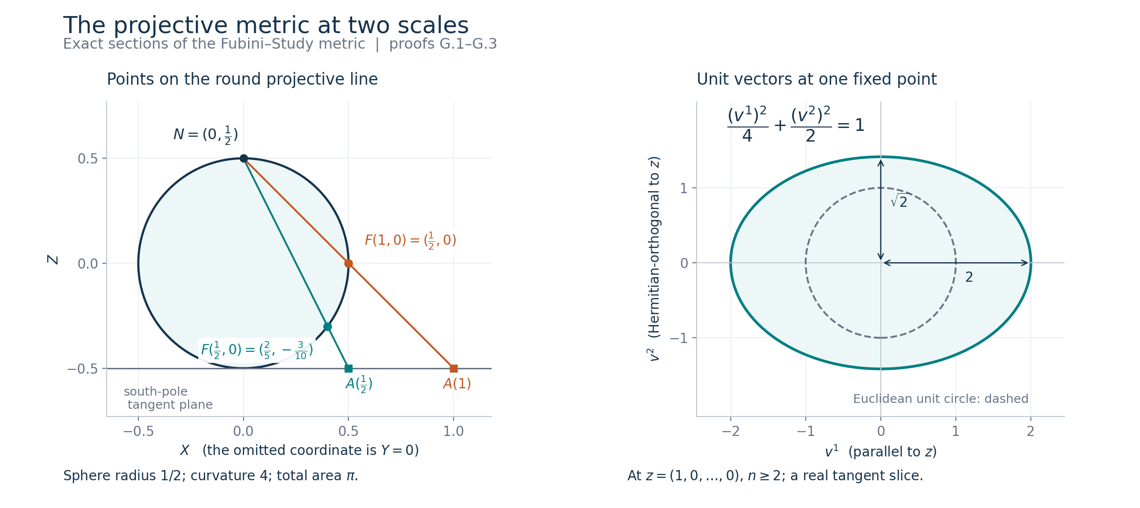
Left: the radius-one-half meridian circle, its north pole, the two exact points F(1/2,0) and F(1,0), and their projection rays to the south-pole tangent plane. Right: the Fubini–Study unit-vector ellipse at z=(1,0,...,0) in the real v1,v2 tangent slice, with semiaxes 2 and square root of 2; a dashed Euclidean unit circle provides the comparison.

Figure G.1. The left panel plots the $X,Z$ meridian and the exact points in (G.7); its omitted ambient coordinate is $Y=0$. The right panel plots (G.8) in one tangent space, with the radial and Hermitian-orthogonal directions labelled. The geometry and scale are proved in G.1–G.3. Reproducible plotting source.

H. Quotients and inherited metrics

Theorem H.1 (flat complex tori for every full lattice). Let $v_1,\ldots,v_{2n}$ be a real basis of $\mathbb C^n$ and let $\Lambda=\sum_j\mathbb Z v_j$. Then $T=\mathbb C^n/\Lambda$ is a compact complex manifold. Every constant positive Hermitian metric on $\mathbb C^n$ descends to a complete flat Kähler metric on $T$. The standard complex tensor always descends; the map $z\mapsto iz$ descends to the quotient precisely when $i\Lambda\subset\Lambda$.

Proof. For $n=0$ the quotient is a single point and all assertions are immediate. Suppose $n\geq1$. Let $B:\mathbb R^{2n}\to\mathbb C^n$ be the real isomorphism with columns $v_j$. Its bounded inverse, as a finite-dimensional linear map Local tools 0.2, gives $|Bm|\geq\|B^{-1}\|^{-1}|m| \quad(m\in\mathbb R^{2n}).$ Thus nonzero lattice vectors have a uniform positive lower norm bound $\delta=\|B^{-1}\|^{-1}$, and only finitely many lie in any bounded set: their integer coordinate vectors lie in a bounded box, which contains finitely many integer vectors. In particular $\Lambda$ is closed; if a sequence of its points converges, its tail lies in a fixed bounded box and hence takes only finitely many values.

The quotient map $q$ is open, since the inverse image of the image of an open set is its union of lattice translates. Every ball of radius less than $\delta/3$ maps injectively to the quotient: two of its points have distance less than $2\delta/3$, so cannot differ by a nonzero lattice vector. The restriction of $q$ is an open continuous bijection onto its image and gives a chart.

The quotient is Hausdorff. If $z-w\notin\Lambda$, then $\eta=\inf_{\lambda\in\Lambda}|z-w-\lambda|>0$: only finitely many lattice vectors can have $|z-w-\lambda|\leq |z-w|+1$, so the infimum in that bounded range is a positive minimum, and vectors outside it cannot lower the infimum to zero. Balls of radius less than $\eta/3$ around $z,w$ have disjoint images. Images of a countable Euclidean basis form a countable basis for the quotient, because $q$ is open. Thus these are charts on a Hausdorff second-countable manifold.

On chart overlaps their inverse lifts differ by a lattice vector. That vector is locally constant: it depends continuously on the point and any two distinct lattice vectors are at least $\delta$ apart. Hence every transition is locally a translation. It is holomorphic by A.2, giving a complex atlas. Every orbit has a representative $B(t_1,\ldots,t_{2n})$ with $0\leq t_j\leq1$, by subtracting the integer parts of its real coordinates. This parallelepiped is compact Local tools 0.1, and its continuous image is the whole quotient, so $T$ is compact.

A constant positive Hermitian metric, its tensor $J_0$, and its fundamental form are invariant under translations. They therefore agree in overlapping lifted charts and descend. The form has constant coefficients there, hence is closed. D.2 makes the descended metric Kähler. Its Levi-Civita coefficients in each lifted real chart are zero by Riemannian connections A.1, so the curvature is zero by its definition as the commutator of covariant derivatives.

For any initial position and velocity in the quotient, choose a lift $z$ and its corresponding velocity $u$. The curve $t\mapsto q(z+tu)$ is a geodesic for all real $t$, since in every local lifted chart its acceleration is zero. Local geodesic uniqueness is proved in Geodesics A.1. Thus every maximal geodesic extends for all time. The equivalence with metric completeness is Hopf–Rinow B.2.

For the map $z\mapsto iz$, equality of the images of $z$ and $z+\lambda$ requires and is implied by $i\lambda\in\Lambda$ for all $\lambda$. This proves the last criterion. If the inclusion holds, multiplying it again by $i$ gives $-\Lambda\subset i\Lambda$, hence equality, so it even gives a quotient automorphism. The tensor's descent only used the identity derivative of translations and imposes no such condition. Rank zero gives the one-point torus. □

Theorem H.2 (Kähler metrics under holomorphic immersion). A holomorphic immersion $f:M\to M'$ into a Kähler manifold induces a Kähler metric on $M$. Completeness of the ambient manifold alone does not imply completeness of the induced metric.

Proof. The complex atlases make the domain's $J$ integrable. Since $df$ is injective, $g(X,Y)=g'(dfX,dfY)$ is a smooth positive metric. The intertwinement $df\circ J=J'\circ df$ is A.3. It gives $J$-invariance and $\omega(X,Y)=g(JX,Y) =\omega'(dfX,dfY)=(f^*\omega')(X,Y).$ Exterior differentiation commutes with smooth pullback, including its chain-rule proof in the exterior-calculus prerequisites of Curvature A.1. Thus $d\omega=f^*d\omega'=0$. D.2 proves the assertion.

For the completeness issue take the inclusion of the unit disc in $\mathbb C$, with the ambient Euclidean metric. This is a holomorphic immersion and its induced metric is Euclidean on the disc. The geodesic $\gamma(t)=t$ starting at zero with real unit velocity reaches its boundary as $t\uparrow1$. A continuous extension at $t=1$ within the disc would have to have value $1$ in the ambient plane, which is not in the disc. Local geodesic uniqueness therefore precludes a complete continuation. The ambient Euclidean plane is complete: a Euclidean Cauchy sequence converges coordinatewise by Local tools 0.1. This proves the claimed limitation by a concrete example. □

I. The octonionic almost complex six-sphere

The algebra used here has already been constructed with full proofs in De Rham decomposition Y.1 and Z.1. Its quaternion basis obeys $ij=k,\ jk=i,\ ki=j$ and $i^2=j^2=k^2=-1$. On $\mathbb O=\mathbb H\oplus\mathbb H$ the convention is $(a,b)(c,d)=(ac-\bar d\,b,\ da+b\bar c),\qquad \overline{(a,b)}=(\bar a,-b). \tag{I.1}$ The identity is $1=(1,0)$; the norm is $|(a,b)|^2=|a|^2+|b|^2$. De Rham Z.1 proves multiplicativity of this norm, conjugation reversing products, alternativity, and the adjoint identities $L_u^*=L_{\bar u}$, $R_u^*=R_{\bar u}$. These are exact programme proof providers, so no external reference is being substituted for an algebraic identity.

Lemma I.1 (a seven-dimensional cross product). On $V=1^\perp=\operatorname{Im}\mathbb O$, define $u\times v=uv+\langle u,v\rangle1. \tag{I.2}$ This is a bilinear alternating operation with values in $V$. It satisfies $\begin{aligned} \langle u\times v,u\rangle&=\langle u\times v,v\rangle=0,\\ |u\times v|^2&=|u|^2|v|^2-\langle u,v\rangle^2,\\ u\times(u\times v)&=-|u|^2v+\langle u,v\rangle u. \end{aligned} \tag{I.3}$ The trilinear form $\Phi(u,v,w)=\langle u\times v,w\rangle$ is alternating.

Proof. For imaginary $u$, De Rham Z.1 gives $u^2=-|u|^2\,1$, $L_u^*=-L_u$, and $L_u^2=-|u|^2I$. Polarizing the quadratic identity gives $uv+vu=-2\langle u,v\rangle1.$ Conjugation reverses the product and sends $u,v$ to $-u,-v$, so $\overline{uv}=vu$. Its real part is therefore $-\langle u,v\rangle$; (I.2) is its imaginary part. The same sum identity makes it alternating.

For imaginary $u,v,w$, its scalar correction is perpendicular to $w$. Skew-adjointness of $L_u$ gives $\langle u\times v,w\rangle =\langle uv,w\rangle=-\langle v,uw\rangle =-\langle v,u\times w\rangle.$ Thus $\Phi$ changes sign when its last two arguments are exchanged. Alternation of the cross product gives the sign change in its first two arguments. These exchanges generate all permutations, so $\Phi$ is alternating. In particular the two orthogonality assertions follow by repeating an argument.

The real and imaginary parts of $uv$ are perpendicular. Norm multiplicativity therefore gives $|u|^2|v|^2=|uv|^2 =\langle u,v\rangle^2+|u\times v|^2.$ Finally, $\langle u,u\times v\rangle=0$ implies that $u\times(u\times v)=u(u\times v)$. The multiplication-operator identity in De Rham Z.1, which does not reassociate arbitrary octonions, gives $u(u\times v)=u(uv)+\langle u,v\rangle u =-|u|^2v+\langle u,v\rangle u.$ This proves every identity in (I.3). □

Lemma I.2 (the basis and its multiplication signs). Put $\begin{gathered} e_1=(i,0),\quad e_2=(j,0),\quad e_3=(k,0),\quad e_4=(0,1),\\ e_5=(0,i),\quad e_6=(0,j),\quad e_7=(0,k). \end{gathered} \tag{I.4}$ They are an orthonormal basis of $V$. All products of distinct basis vectors are specified by the seven oriented triples $(1,2,3),\ (1,4,5),\ (2,4,6),\ (3,4,7),\ (1,7,6),\ (2,5,7),\ (3,6,5). \tag{I.5}$ For a displayed triple $(a,b,c)$, the products $e_a e_b=e_c,\ e_b e_c=e_a,\ e_c e_a=e_b$ hold; reversing an ordered pair changes the sign. The same table is the cross-product table on distinct basis vectors.

Proof. Orthonormality is the Euclidean norm of (I.1). Every $e_a$ is imaginary, so its square is $-1$ by De Rham Z.1; I.1 gives anticommutation for orthogonal imaginary vectors. To verify all of the signs, let $a_0=1,a_1=i,a_2=j,a_3=k$, and put $f_s=(0,a_s)$, $0\leq s\leq3$. Formula (I.1) says, for $1\leq r\leq3$, $\begin{aligned} e_r f_s&=(0,a_s a_r),& f_s e_r&=(0,a_s\bar a_r)=-(0,a_s a_r),\\ f_s f_t&=(-\bar a_t a_s,0). \end{aligned} \tag{I.6}$ Together with the proved quaternion products De Rham Y.1, these cover every pair. More explicitly, the three cyclic products for each row of (I.5) are respectively $\begin{array}{c|ccc} (1,2,3)&e_1e_2=e_3&e_2e_3=e_1&e_3e_1=e_2\\ (1,4,5)&e_1e_4=e_5&e_4e_5=e_1&e_5e_1=e_4\\ (2,4,6)&e_2e_4=e_6&e_4e_6=e_2&e_6e_2=e_4\\ (3,4,7)&e_3e_4=e_7&e_4e_7=e_3&e_7e_3=e_4\\ (1,7,6)&e_1e_7=e_6&e_7e_6=e_1&e_6e_1=e_7\\ (2,5,7)&e_2e_5=e_7&e_5e_7=e_2&e_7e_2=e_5\\ (3,6,5)&e_3e_6=e_5&e_6e_5=e_3&e_5e_3=e_6 . \end{array} \tag{I.7}$ Each entry with an $f_s$ follows by its indicated substitution in (I.6), and the first row is quaternion multiplication. The seven triples contain all $21$ unordered pairs of distinct indices, without repetition. Thus (I.7), its reversed products, and the squares determine the entire bilinear multiplication table. The scalar correction in (I.2) is zero on distinct basis vectors, giving the cross-product assertion. □

Theorem I.3 (the full obstruction on the unit six-sphere). On $S^6=\{p\in V:|p|=1\}$, set $J_pU=p\times U,\qquad U\in T_pS^6=p^\perp. \tag{I.8}$ This is a smooth orthogonal almost complex structure for the round metric. Its Levi-Civita derivative is $A_p(U,V):=(\nabla_UJ)V =U\times V-\langle JU,V\rangle p. \tag{I.9}$ Its Nijenhuis tensor is $\begin{aligned} N_J(U,V)&=-4J A_p(U,V),\\ |N_J(U,V)|^2 &=16\bigl(|U|^2|V|^2-\langle U,V\rangle^2 -\langle JU,V\rangle^2\bigr). \end{aligned} \tag{I.10}$ At every point there are orthonormal tangent $U,V$ with $|N_J(U,V)|=4$. Thus this particular almost complex structure is not integrable on any nonempty open subset.

Proof. The differential of $p\mapsto |p|^2$ is $U\mapsto2\langle p,U\rangle$, nonzero on the unit level; Local tools 1.3 gives its smooth tangent bundle with $T_pS^6=p^\perp$. I.1 makes $p\times U$ tangent and gives $p\times(p\times U)=-U,\qquad |p\times U|^2=|U|^2.$ Polarizing the latter equality gives metric compatibility. The coefficients are bilinear in $p,U$, so the field is smooth.

For tangent fields let $D$ denote the ambient Euclidean derivative and let $P_pW=W-\langle W,p\rangle p$ be orthogonal projection to $p^\perp$. The derivative $P D$ on tangent fields is metric compatible, since normal components pair to zero with tangent vectors. It has zero torsion: the ambient derivative difference $D_UV-D_VU=[U,V]$ is the tangent bracket Principal bundles C.3, and projection fixes it. Uniqueness in Riemannian connections A.1 identifies $PD$ with the round Levi-Civita derivative.

Differentiate $J_pV=p\times V$ in direction $U$. Bilinearity gives $U\times V+p\times D_UV$. Subtract $p\times\nabla_UV$. The remaining contribution from $D_UV-\nabla_UV$ is a multiple of $p\times p=0$. Tangential projection therefore gives $A_p(U,V)=P_p(U\times V).$ By the alternating form in I.1, $\langle U\times V,p\rangle=\Phi(U,V,p)=\Phi(p,U,V)=\langle JU,V\rangle$. This proves (I.9), in particular $A(U,V)=-A(V,U)$.

Differentiate $J^2=-I$ using the tensor derivative product rule Linear and affine connections C.1: $A(U,JV)=-J A(U,V).$ Skewness then also gives $A(JU,V)=-A(V,JU)=J A(V,U)=-J A(U,V). \tag{I.11}$ For any torsion-free connection, substituting $[X,Y]=\nabla_XY-\nabla_YX$ in the definition of $N_J$ and applying the product rule gives $N_J(U,V) =A(JU,V)-A(JV,U)+J A(V,U)-J A(U,V). \tag{I.12}$ To check cancellation, the first bracket contributes $A(JU,V)-A(JV,U)+J\nabla_{JU}V-J\nabla_{JV}U$. The next two brackets contribute respectively $-J\nabla_{JU}V+JA(V,U)-\nabla_VU$ and $-JA(U,V)+\nabla_UV+J\nabla_{JV}U$. The final term contributes $-\nabla_UV+\nabla_VU$. All displayed vector derivatives cancel, leaving (I.12).

Now (I.11) and skewness make each of its four terms equal to $-JA(U,V)$, with the written signs included. This proves $N_J=-4JA$. Since $J$ is an isometry and $A$ is the orthogonal projection of $U\times V$, $|A(U,V)|^2=|U\times V|^2-\langle JU,V\rangle^2.$ I.1 gives the second formula of (I.10).

At any point choose a unit tangent vector $U$. The vectors $U,JU$ are orthonormal: their norms agree and $J$ is skew for the metric by D.1. Their orthogonal complement inside the six-dimensional tangent space has dimension four, by extension of an orthonormal basis Principal bundles D.2. Choose a unit $V$ there. Then (I.10) gives $|N_J(U,V)|^2=16$. B.2 says that every complex atlas inducing $J$ would make this tensor vanish. It follows that no such atlas exists on any nonempty open set. This conclusion concerns the field (I.8), not every possible almost complex structure on the sphere. □

Example I.4 (an independent calculation with tangent brackets). At $p=e_7$, in the convention (I.4), one has $N_J(e_1,e_2)=-4e_4$. This value can be computed directly from tangent-field brackets, without using the covariant derivative formula (I.12).

Proof. For a fixed imaginary vector $a$, define two polynomial expressions restricted to the unit sphere: $U_a(q)=a-\langle a,q\rangle q,\qquad K_a(q)=q\times a. \tag{I.13}$ Both are tangent, and $JU_a=K_a$ because $q\times q=0$. Their derivatives along a tangent vector $W$ are $D_WU_a=-\langle a,W\rangle q-\langle a,q\rangle W,\qquad D_WK_a=W\times a. \tag{I.14}$ These are derivatives of the explicit ambient polynomial maps, hence also compute derivatives of their restrictions along any sphere curve.

Take $U=U_{e_1}$, $V=U_{e_2}$. At $p=e_7$, (I.7) gives $U=e_1,\qquad V=e_2,\qquad JU=-e_6,\qquad JV=e_5,\qquad Je_3=e_4.$ Using $[X,Y]=D_XY-D_YX$, formula (I.14) now gives, with all values at $p$, $\begin{aligned} [U,V]&=0,\\ [JU,V]&=0-e_2\times e_1=e_3,\\ [U,JV]&=e_1\times e_2-0=e_3,\\ [JU,JV]&=(-e_6)\times e_2-e_5\times e_1=-2e_4. \end{aligned} \tag{I.15}$ For the final line, $e_6e_2=e_4$ and $e_5e_1=e_4$ are the third entries in the $(2,4,6)$ and $(1,4,5)$ rows. For the first three lines the derivative terms of $U_a$ are zero because the relevant coordinate pairings at $e_7$ vanish. Every result is tangent, as the formulas also show directly.

Substitution of these four bracket values into the definition of $N_J$ gives $N_J(e_1,e_2)=-2e_4-Je_3-Je_3-0=-4e_4.$ It agrees with I.10, since $A(e_1,e_2)=e_3$. I.3 supplies the all-point nonvanishing, and B.2 supplies the necessary vanishing for an integrable structure. Thus the direct bracket computation and the tensor-norm argument prove complementary parts of the obstruction. □

Corollary I.5 (the round fundamental form is nowhere closed). For the almost complex structure of I.3 and its round metric, $d\omega_p(U,V,W)=3\langle U\times V,W\rangle \quad(U,V,W\in T_pS^6). \tag{I.16}$ At every $p$ there are unit tangent vectors on which this three-form has value $3$. In particular $d\omega_{e_7}(e_1,e_2,e_3)=3$.

Proof. The tensor rule and metric compatibility give $(\nabla_U\omega)(V,W)=\langle(\nabla_UJ)V,W\rangle$. By I.3, $(\nabla_UJ)V$ is the tangential projection of $U\times V$; its normal part pairs to zero with the tangent vector $W$. Formula (D.2) now expresses $d\omega(U,V,W)$ as the cyclic sum of $\langle U\times V,W\rangle$. The alternating identity of I.1 makes the three cyclic terms equal, proving (I.16).

At any $p$, choose the unit orthogonal vectors $U,V$ from the final paragraph of I.3, with $V\perp JU$. The cross product $U\times V$ has norm one by I.1, and its component along $p$ is $\langle JU,V\rangle=0$ by I.3. Thus $W=U\times V$ is a unit tangent vector and (I.16) has value $3$. At $p=e_7$, I.2 gives $e_1\times e_2=e_3$, yielding the specified value. A three-form nonzero at every point cannot vanish on any nonempty open set, so the fundamental form is nowhere closed in this sense. □

J. Preparing coordinates for the smooth integrability theorem

In this part $J$ is smooth and $N_J=0$. Thus B.2–B.3 give involutivity of both eigenbundles and $d=\partial_J+\bar\partial_J,\qquad \partial_J^2=\bar\partial_J^2=0,\qquad \partial_J\bar\partial_J=-\bar\partial_J\partial_J. \tag{J.1}$ Subscripts distinguish these operators from the ordinary coordinate derivatives before complex coordinates have been obtained.

Lemma J.1 (arbitrary finite coordinate normalization). At any point of a smooth almost complex manifold with $N_J=0$, and for every integer $s\geq1$, there are smooth real coordinates, written as a complex tuple $z$, in which $T^{0,1}_J =\operatorname{span}_{\mathbb C}\{L_1,\ldots,L_n\},\qquad L_j=\partial_{\bar z^j}+\sum_a A_j^a(z)\partial_{z^a}, \qquad A(z)=O(|z|^s). \tag{J.2}$ Every real derivative of order $k\leq s$ of $A$ is $O(|z|^{s-k})$. The coordinate differential at the chosen point is complex linear for $J$.

Proof. The zero-dimensional case has no equations. Otherwise choose the real paired basis of B.1 at the point, use a real chart with that differential, and put the point at zero. Then $J(0)$ is the standard complex matrix. Projection of $T^{0,1}_J$ onto the coordinate $(0,1)$ space is invertible at zero and, by continuity of the determinant, nearby. Its inverse supplies the frame in (J.2), with $A(0)=0$. The coefficients are smooth by matrix inversion Local tools 0.4.

The bracket $[L_j,L_k]$ has no coordinate $\partial_{\bar z}$ component. Involutivity places it in the span of the $L_a$, whose $\partial_{\bar z}$ components are the standard basis. Consequently the bracket is zero. Its remaining coefficients give $\partial_{\bar z^j}A_k^a-\partial_{\bar z^k}A_j^a +\sum_b\bigl(A_j^b\partial_{z^b}A_k^a -A_k^b\partial_{z^b}A_j^a\bigr)=0. \tag{J.3}$

Suppose the Taylor terms of $A$ below degree $s$ vanish. Write its homogeneous term of degree $s$ as $P_j^a(z,\bar z)$. These are polynomials in $z,\bar z$, because the real coordinates are their linear combinations. The nonlinear terms in (J.3) have order at least $2s-1$. Since $2s-1>s-1$, the degree $s-1$ terms give the polynomial identities $\partial_{\bar z^j}P_k^a=\partial_{\bar z^k}P_j^a.$ Treat the two sets of polynomial variables independently and put $Q^a(z,\bar z)=\int_0^1 \sum_k\bar z^kP_k^a(z,t\bar z)\,dt. \tag{J.4}$ This is a homogeneous polynomial of total degree $s+1$. Differentiating it with respect to $\bar z^j$, and using the preceding identity, gives $\begin{aligned} \partial_{\bar z^j}Q^a &=\int_0^1\left(P_j^a(z,t\bar z) +t\sum_k\bar z^k \partial_{\bar z^k}P_j^a(z,t\bar z)\right)\,dt\\ &=\int_0^1\frac{d}{dt}\bigl[tP_j^a(z,t\bar z)\bigr]\,dt =P_j^a(z,\bar z). \end{aligned} \tag{J.5}$ All these integrals are finite polynomial integrals; the fundamental theorem is Local tools 0.3.

Make the real coordinate change $w^a=z^a-Q^a(z,\bar z)$. Its differential at zero is the identity, so Local tools 1.2 makes it a smooth local diffeomorphism. Direct differentiation shows $L_jw^a=A_j^a-P_j^a-\sum_b A_j^b\partial_{z^b}Q^a =O(|z|^{s+1}). \tag{J.6}$ Here the last sum has order $2s\geq s+1$. Meanwhile $L_j\bar w^k=\delta_{jk}+O(|z|^s)$. Inverting this latter matrix renormalizes the frame so that its $\partial_{\bar w}$ part is again the identity. Its $\partial_w$ coefficients still have order $s+1$. The norms of $w$ and $z$ are comparable near zero, since their differentials there agree. Thus the same order holds in the new coordinates.

Start with $s=1$ and repeat finitely many times. Each change has identity differential at zero, so the original complex-linear differential is preserved. Finally, the derivative estimates follow from Taylor's formula, not just from differentiating an unspecified order bound. For a smooth coefficient with all terms below degree $s$ zero, apply the one-variable integral Taylor formula to its restriction along the segment from zero to $z$; applying the same formula to each derivative of order $k\leq s$ bounds it by a constant times $|z|^{s-k}$. This segment formula follows by repeated integration of the fundamental theorem. The derivatives on a fixed smaller closed ball are bounded, which gives the required constants. □

Lemma J.2 (a positive potential and uniformly controlled logarithmic weights). Take J.1 with $s=3$, set $\psi=|z|^2$, and shrink the coordinate ball. The real form $\omega=i\partial_J\bar\partial_J\psi \tag{J.7}$ is positive, closed and of type $(1,1)$. Its associated real metric is parallel with respect to $J$. If $F$ is any smooth real $(1,1)$-form on a neighbourhood of a closed smaller ball $|z|\leq R$, there is a constant $a>0$, independent of $0<\varepsilon\leq1$, such that $\begin{aligned} \Phi_\varepsilon&=a\psi+(n+1)\log(\psi+\varepsilon^2),\\ F+i\partial_J\bar\partial_J\Phi_\varepsilon&\geq\omega \qquad (|z|<R). \end{aligned} \tag{J.8}$

Proof. The real logarithm and exponential, their derivatives and their inverse and product identities are the integral constructions proved in Local tools 0.5. Positivity means $\omega(X,JX)>0$ for nonzero real $X$. In the ordinary coordinates let $\omega_0=i\sum_j dz^j\wedge d\bar z^j$; its real metric is twice the Euclidean metric. The graph description (J.2) expresses the two type projections as smooth matrix functions of $A,\bar A$, equal to the ordinary projections when $A=0$. J.1 and matrix inversion therefore give projection errors of order $r^3$, with first and second derivatives of orders $r^2,r$, where $r=|z|$. As $d\psi$ has coefficients of order $r$, $\begin{aligned} \bar\partial_J\psi-\bar\partial_0\psi&=O(r^4),\\ \omega-\omega_0&=O(r^3),& D(\omega-\omega_0)&=O(r^2). \end{aligned} \tag{J.9}$ For the second line differentiate the first, and also account for the order $r^3$ error of the outer type projection acting on a bounded two-form. The next derivative uses the corresponding differentiated coefficient bounds. These arguments concern actual smooth coefficients in the fixed chart.

The leading positive matrix is constant. The small error in (J.9) preserves positivity on a sufficiently small ball, by the positive lower bound on its unit sphere. Reality follows by conjugating (J.7) and using (J.1). The same identities give $d\omega=0$. D.1 supplies its real compatible metric, and D.2, with the already assumed $N_J=0$, proves that its Levi-Civita connection preserves $J$. No complex atlas has been inferred here.

For a $(1,0)$-covector $\alpha$, use the Hermitian norm induced by the complexified real metric: in a coframe with $\omega=i\sum_j\theta^j\wedge\bar\theta^j$, the squared norm of $\sum a_j\theta^j$ is $\sum|a_j|^2$. A unitary coframe exists by F.1. In that frame the finite-dimensional Cauchy–Schwarz inequality gives $i\alpha\wedge\bar\alpha\leq|\alpha|_\omega^2\,\omega. \tag{J.10}$ For $\alpha=\partial_J\psi$, (J.9) and the inverse-matrix formula give $|\partial_J\psi|_\omega^2=\psi+O(r^5). \tag{J.11}$ Indeed its coefficient error relative to $\partial_0\psi$ is $O(r^4)$, its leading coefficients are $O(r)$, and the inverse metric differs from the constant inverse by $O(r^3)$. Every error in the squared norm is therefore $O(r^5)$ or smaller.

The chain rule, (J.7) and (J.10) now imply $\begin{aligned} i\partial_J\bar\partial_J\log(\psi+\varepsilon^2) &=\frac{\omega}{\psi+\varepsilon^2} -\frac{i\partial_J\psi\wedge\bar\partial_J\psi} {(\psi+\varepsilon^2)^2}\\ &\geq\frac{\varepsilon^2-Cr^5}{(r^2+\varepsilon^2)^2}\,\omega \geq-Cr\,\omega . \end{aligned} \tag{J.12}$ The last inequality uses $r^5/(r^2+\varepsilon^2)^2\leq r$, including $r=0$. It is uniform in $\varepsilon$.

On the closed smaller ball $F\geq-B\omega$ for some $B\geq0$: in finitely many smooth frames its coefficients are bounded and the positive metric has a uniform lower bound. Take $a\geq B+1+(n+1)CR$. Substituting (J.12) proves (J.8). All matrix bounds come from compactness and the finite-dimensional norm estimates in Local tools 0.1–0.2. □

Lemma J.3 (a complete metric with explicit small-gradient cutoffs). On a smaller ball $\Omega=\{\psi<R^2\}$, the form $\gamma=\omega+i\partial_J\bar\partial_J b,\qquad b=-\log(R^2-\psi) \tag{J.13}$ defines a complete positive metric preserving $J$. There are smooth functions $\chi_k$ with compact support in $\Omega$, between zero and one, equal to one on successively larger compact subsets exhausting $\Omega$, such that $|d\chi_k|_\gamma\leq C/k. \tag{J.14}$

Proof. Choose the closed ball inside the positive-coordinate neighbourhood from J.2. The chain rule gives $\gamma=\left(1+\frac1{R^2-\psi}\right)\omega +\frac{i\partial_J\psi\wedge\bar\partial_J\psi} {(R^2-\psi)^2}. \tag{J.15}$ It is real, closed and positive. D.2 again proves parallelness. For real $X$, the last term evaluated on $(X,JX)$ is $2|\partial_J\psi(X)|^2/(R^2-\psi)^2$. Since $d\psi(X)=2\operatorname{Re}\partial_J\psi(X)$, the associated real metric obeys $|X|_\gamma^2\geq\tfrac12|db(X)|^2,\qquad |db|_\gamma\leq\sqrt2. \tag{J.16}$

Here is a direct completeness proof. On the closed ball the metric of $\omega$ bounds a fixed positive multiple of the Euclidean metric below. As $\gamma\geq\omega$, a Cauchy sequence for the length distance of $\gamma$ is Euclidean Cauchy and has a limit in the closed ball. Along any piecewise smooth curve (J.16) gives a bound of $\sqrt2$ times its length for the change in $b$. Taking infima over such curves shows that $b$ is $\sqrt2$-Lipschitz for that distance. It is consequently bounded on the Cauchy sequence. The limit cannot lie on the boundary, where $b$ tends to infinity. At an interior limit, the metric is bounded above on a small convex coordinate ball; straight segments then show convergence also in the $\gamma$ distance. This proves metric completeness using the real completeness theorem Local tools 0.1.

Set $\rho=b-b(0)$. It is nonnegative and proper on $\Omega$. To obtain a smooth nonincreasing function $\eta:\mathbb R\to[0,1]$ equal to one on $(-\infty,1]$ and zero on $[2,\infty)$, choose a nonzero nonnegative smooth bump $\beta$ supported in $(1,2)$, by Local tools 3.1, and put $\eta(t)=(\int\beta)^{-1}\int_t^\infty\beta(s)\,ds$. The integral is over a fixed compact interval; the fundamental theorem proves smoothness and $\eta'=-\beta/\int\beta\leq0$. Put $\chi_k=\eta(\rho/k)$. Its support is contained in the compact sublevel $\rho\leq2k$, and it equals one where $\rho\leq k$. These sublevels exhaust $\Omega$. Finally the chain rule and (J.16) give (J.14), with $C=\sqrt2\sup|\eta'|$. The sequence is nondecreasing because $\eta$ is nonincreasing. □

Lemma J.4 (the weighted equation that suffices for coordinates). In the normalized ball of J.2 let $\chi$ be a smooth compactly supported function equal to one near zero, and put $g_j=\bar\partial_J(\chi z^j). \tag{J.17}$ These are smooth compactly supported closed $(0,1)$-forms. For the weights in (J.8), their squared weighted integrals are bounded uniformly as $\varepsilon\downarrow0$. Suppose smooth functions $u_j$ have been obtained on $\Omega$ with $\bar\partial_Ju_j=g_j,\qquad \int_{\Omega\setminus\{0\}} |u_j|^2 e^{-a\psi}|z|^{-2n-2}\,d\mu_\omega<\infty. \tag{J.18}$ Then $w^j=\chi z^j-u_j$ are complex coordinates for $J$ near zero. In particular the existence and smoothness of solutions satisfying (J.18) suffice for the full smooth integrability conclusion.

Proof. Closedness is $\bar\partial_J^2=0$ from (J.1). Near zero, (J.2) gives $\bar\partial_J z^j=O(r^3)$, so $|g_j|_\omega\leq Cr^3$. The smooth density of $\omega$ is bounded above and below on the closed ball. Its coordinate-independent integration is Killing fields F.1. For the possibly improper positive integrals here, the integral means the supremum of compactly supported cutoff integrals; this convention agrees with ordinary integration whenever the integrand has compact support.

To check convergence without assuming a polar-coordinate integration formula, divide a small punctured ball into dyadic shells with radii comparable to $t_m=2^{-m}r_0$. Each shell is contained in a box of volume $C t_m^{2n}$. On it, $|g_j|_\omega^2 e^{-\Phi_\varepsilon} \leq C t_m^6 t_m^{-2n-2} = C t_m^{4-2n}. \tag{J.19}$ The constants account for the factor two between the inner and outer radii. Each shell integral is thus at most $C t_m^4$, and the geometric sum is finite uniformly in $\varepsilon$. One may obtain the same bound for continuous integrals by covering each shell with boxes inside a shell enlarged by fixed factors. Such covers can be obtained by rescaling a single finite box cover of the closed unit shell; they have bounded overlap. At every positive inner cutoff only finitely many shells occur, so the bound passes to the supremum defining the improper integral. For each fixed positive $\varepsilon$ the integrand is smooth at zero; removing a box of side tending to zero changes its integral by at most its bound on a fixed box times the removed volume. Thus the punctured and unpunctured integrals agree. Away from zero all weights are uniformly bounded on the support of $g_j$. This proves the asserted uniform estimate.

Now (J.18) forces both $u_j(0)=0$ and $du_j(0)=0$. If the value were nonzero, it would have a fixed positive lower bound near zero. Choose a closed box $Q$ lying in a small annular sector, with positive volume, whose dilates $2^{-m}Q$ are disjoint and approach zero. On the $m$-th box the weighted integral would then be bounded below by $c\,2^{2m}$. Finite unions of these boxes contradict the finite integral; smooth inner cutoffs give the same lower bounds up to a fixed positive factor.

If the value is zero but the real differential is nonzero, there is a real unit direction on which it is nonzero. Continuity of that linear map bounds its modulus below on an open cone about that direction. Differentiability, uniformly for directions in a smaller cone, gives $|u_j(z)|\geq c|z|$ there for small $|z|$. Choose $Q$ in that smaller cone. The factor $|u_j|^2$ now contributes at least $c\,2^{-2m}$, exactly canceling the preceding factor $2^{2m}$. Every scaled box contributes a fixed positive amount, again a contradiction. The density and $e^{-a\psi}$ have fixed positive lower bounds in these estimates.

Thus $dw(0)=dz(0)$ and $\bar\partial_Jw=0$. The real inverse theorem Local tools 1.2 gives a smooth local diffeomorphism. The equation $\bar\partial_Jw=0$ says its differential intertwines $J$ with the standard complex structure. Every transition between two such charts has complex-linear differential; A.2–A.3 make it holomorphic. Therefore these are the required complex charts. This lemma is conditional on (J.18). Parts K–M establish the analytic prerequisites, and N.1 constructs functions satisfying that condition. □

K. Hilbert spaces and domains for the weighted equation

Inner products in this part are complex linear in the first argument. A Hilbert space is an inner-product space complete for its norm. An adjoint below is the adjoint of an operator with its specified domain; it is not automatically the formal integration-by-parts expression.

Lemma K.1 (completion, projection and representation). Every complex inner-product space has a Hilbert completion. If $M$ is a closed linear subspace of a Hilbert space $H$, every $x\in H$ has a unique decomposition $x=m+e$, with $m\in M$ and $e\perp M$; both projections have norm at most one. Every bounded complex-linear functional $\ell$ on $H$ has the form $\ell(x)=\langle x,w\rangle,\qquad \|\ell\|=\|w\|, \tag{K.1}$ for a unique $w\in H$.

Proof. First the inner-product axioms imply Cauchy–Schwarz. For $y\ne0$, substitute $\lambda=\langle x,y\rangle/\|y\|^2$ in $0\leq\|x-\lambda y\|^2$. Expansion gives $|\langle x,y\rangle|^2\leq\|x\|^2\|y\|^2$. The case $y=0$ is immediate. The triangle inequality follows by expanding $\|x+y\|^2$ and applying this bound.

For the completion take Cauchy sequences $(x_j)$ and identify two when the norm of their difference tends to zero. Addition and scalar multiplication preserve this relation. Cauchy–Schwarz shows that $\langle x_j,y_j\rangle$ is a scalar Cauchy sequence: both vector sequences are bounded, and $|\langle x_j,y_j\rangle-\langle x_k,y_k\rangle| \leq\|x_j-x_k\|\|y_j\|+\|x_k\|\|y_j-y_k\|.$ Its limit defines an inner product on the quotient. A class has zero norm precisely when its representative tends to zero in norm, so this inner product is positive definite. Constant sequences embed the original space isometrically and densely.

To verify completeness explicitly, for a Cauchy sequence $X_j$ of classes choose original vectors $x_j$ with $\|X_j-x_j\|<2^{-j}$, using that density. The sequence $(x_j)$ is Cauchy. Its class $X$ satisfies $x_j\to X$: for a fixed index $j$, its distance to $X$ is $\lim_k\|x_j-x_k\|$. The Cauchy property makes this small for large $j$. Hence $X_j\to X$. Scalar limits used here exist by Local tools 0.1.

For projection let $d=\inf_{m\in M}\|x-m\|$, and choose $m_j\in M$ with $\|x-m_j\|\to d$. The parallelogram identity, obtained by expanding the four inner products, gives $\begin{aligned} \|m_j-m_k\|^2 &=2\|x-m_j\|^2+2\|x-m_k\|^2\\ &\quad-4\left\|x-\frac{m_j+m_k}{2}\right\|^2\\ &\leq2\|x-m_j\|^2+2\|x-m_k\|^2-4d^2 . \end{aligned} \tag{K.2}$ Thus $(m_j)$ is Cauchy. Its limit $m$ lies in the closed space $M$ and attains the infimum. For any $v\in M$, the real polynomial $\|x-m-tv\|^2$ is minimized at $t=0$. Its linear coefficient vanishes, so $\operatorname{Re}\langle x-m,v\rangle=0$. Replacing $v$ by $iv$ also makes the imaginary part zero. Therefore $e=x-m\perp M$. Orthogonality gives $\|x\|^2=\|m\|^2+\|e\|^2$, proving the norm bounds. If two decompositions existed, their $M$-components would differ by a vector in both $M$ and $M^\perp$, hence by zero. Applying uniqueness to sums and scalar multiples also proves linearity of the projections.

If $\ell=0$, take $w=0$. Otherwise its kernel $M$ is closed, since $|\ell(x)|\leq\|\ell\|\|x\|$. Choose $q$ with $\ell(q)=1$, and decompose $q=m+e$ as above. Then $\ell(e)=1$ and $e\ne0$. For every $x$, the vector $x-\ell(x)e$ lies in $M$, so $\langle x,e\rangle=\ell(x)\|e\|^2.$ Taking $w=e/\|e\|^2$ proves (K.1). Cauchy–Schwarz bounds its functional norm by $\|w\|$; evaluation at $x=w/\|w\|$ gives equality when $w\ne0$. If two vectors represented the same functional, evaluation on their difference would make its norm zero. This proves uniqueness. In particular a bounded functional on any linear subspace first extends by continuity to its closure, is represented there, and extends to $H$ by its orthogonal projection, with the same norm. □

Lemma K.2 (weak subsequences and the norm bound). Every bounded sequence in a Hilbert space has a weakly convergent subsequence. That is, after passage to a subsequence there is $u$ such that $\langle u_j,v\rangle\longrightarrow\langle u,v\rangle \quad\hbox{for every }v\in H,\qquad \|u\|\leq\liminf_j\|u_j\|. \tag{K.3}$ Here the lower limit is taken along the selected subsequence.

Proof. Let $M$ be the closed linear span of the countable sequence. Apply Gram–Schmidt in its given order, skipping a vector when its residual is zero. At each stage only a finite sum is subtracted. The resulting finite or countable orthonormal family $(e_k)$ has dense span in $M$: every processed vector is in the span already constructed. Pythagoras gives, for every finite $N$, $\sum_{k=1}^N|\langle u_j,e_k\rangle|^2\leq\|u_j\|^2. \tag{K.4}$ Each scalar coefficient is bounded. Repeated subsequence selection using compactness of a real two-dimensional box, Local tools 0.1, followed by the diagonal subsequence, makes all coefficients converge to numbers $c_k$. For a finite family only finitely many selections are necessary.

If the original uniform bound is $C$, (K.4) gives $\sum_{k\leq N}|c_k|^2\leq C^2$ for all $N$. The nonnegative partial sums have a finite supremum and converge to it: otherwise some term would stay a fixed distance below that supremum, contradicting its defining property. Pythagoras makes the partial vector sums $\sum_{k\leq N}c_ke_k$ Cauchy. By completeness they converge to $u\in M$.

Convergence of inner products holds for every finite linear combination of the $e_k$. For $v\in M$, approximate it by such a combination. Cauchy–Schwarz and the uniform bounds on $\|u_j\|,\|u\|$ make the error uniformly small, proving convergence for $v$. For arbitrary $v\in H$, replace it by its projection onto $M$; the orthogonal component pairs to zero with both $u_j$ and $u$. This proves weak convergence.

For every $N$, passage to the limit in the finite sum (K.4) gives $\sum_{k\leq N}|c_k|^2\leq\liminf_j\|u_j\|^2$. Let $N$ increase. The left side tends to $\|u\|^2$, proving (K.3). The proof uses the closed span of the sequence and does not assume that the original Hilbert space is separable. □

Lemma K.3 (weighted completions and weak differential operators). Let $E$ be a smooth finite-rank complex bundle with smooth positive Hermitian metric $h$ on a smooth manifold, and let $\nu$ be a smooth positive density. The inner product $\langle u,v\rangle_{h,\nu} =\int h(u,v)\,\nu,\qquad u,v\in C_c^\infty(E), \tag{K.5}$ has a Hilbert completion $H(E;h,\nu)$. It embeds injectively in weak sections, and multiplication by a smooth fibre map with globally bounded pointwise operator norm extends boundedly to these completions.

If $0\leq\chi_k\leq1$ are smooth compactly supported functions eventually equal to one on each compact set, then $\chi_k u\to u$ in $H$ for every $u\in H$. If additionally the $\chi_k$ are nondecreasing, a smooth section $u$ belongs to $H$ exactly when its positive improper integral $\int h(u,u)\nu$ is finite, and that integral is its squared norm.

For a smooth differential operator $P$ between such bundles, its maximal weak domain $\operatorname{Dom}P_{\max} =\{u\in H(E):Pu\hbox{ is represented by an element of }H(F)\} \tag{K.6}$ defines a closed densely defined operator.

Proof. Compactly supported smooth densities are integrated by finite coordinate partitions and the change-of-variables proof in Killing fields F.1. That construction applies on a noncompact manifold to compact support: only finitely many subordinate charts are needed, and the same overlap calculation proves independence. Its positivity and linearity make (K.5) an inner product. If a nonzero smooth section has nonzero value at one point, continuity and positivity bound its squared norm below by a positive constant on a smaller coordinate box. Thus its integral is positive. K.1 gives the completion.

An element $u$ of the completion assigns to every compactly supported smooth test section $\phi$ the number $\langle u,\phi\rangle$. It is conjugate linear in $\phi$, and bounded by $\|u\|\|\phi\|$. On a fixed compact coordinate set the latter norm is bounded by a constant times the supremum of the coefficient functions of $\phi$. This is a weak section, in the usual sense of a continuous functional on test sections. Equivalently one may use the ordinary coordinate distribution convention: multiplication by the smooth invertible matrix of $h$ and by the smooth positive density converts between the two test pairings. The conversion is invertible on every compact set. If all pairings vanish, $u$ is perpendicular to the dense subspace $C_c^\infty(E)$, so $u=0$. This proves injectivity.

The pointwise bound $|Au|\leq C|u|$, integrated first for smooth compactly supported sections, gives a norm bound $C$ for multiplication. It therefore extends uniquely by completion. In particular multiplication by every $\chi_k$ has norm at most one. On a fixed test section it is eventually the identity. Approximate any $u\in H$ by a test section and apply the norm bound to the difference; this proves $\chi_k u\to u$.

Define a nonnegative improper integral as the supremum of compact cutoff integrals, with cutoff values between zero and one. For a smooth $u$, denote this supremum by $I$. The integrals $I_k=\int\chi_k^2 h(u,u)\nu$ increase to $I$: every compact cutoff is dominated by $\chi_k^2$ once $\chi_k=1$ on its support. If $I<\infty$, then for $m\geq k$, $\|\chi_m u-\chi_k u\|^2 \leq\int(\chi_m^2-\chi_k^2)h(u,u)\nu =I_m-I_k, \tag{K.7}$ because $(b-a)^2\leq b^2-a^2$ for $0\leq a\leq b$. Hence these test sections form a Cauchy sequence in $H$; their weak section is $u$, since they eventually agree with it on every test support. Its squared norm is $\lim I_k=I$. Conversely, if an element of $H$ represents a smooth $u$, the already proved strong convergence of its cutoffs gives $I_k\to\|u\|^2$, so $I=\|u\|^2<\infty$.

The formal adjoint $P^\dagger$ is defined on test sections by ordinary coordinate integration by parts in (K.5). It has smooth coefficients, is a differential operator of the same order, and preserves compact support. In coordinates these assertions follow by repeatedly moving each derivative to the smooth coefficient, density and test function using the product rule and the one-variable fundamental theorem. A partition makes the identity global; uniqueness follows by testing on a section whose coefficients detect any nonzero difference.

Define $Pu$ weakly by $\langle Pu,\phi\rangle=\langle u,P^\dagger\phi\rangle. \tag{K.8}$ It is a continuous functional of finite derivative order on every fixed compact test set. If $u_j\to u$ in $H(E)$ and $Pu_j\to v$ in $H(F)$, then testing (K.8) and passing to the norm limits yields $Pu=v$. This proves closedness of (K.6). Its domain contains every test section, because $P$ maps such a section to a smooth compactly supported one. It is therefore dense. No equality of the Hilbert adjoint with $P^\dagger_{\max}$ has yet been assumed. □

Theorem K.4 (solving a Hilbert complex from an estimate). Let $H_0\xrightarrow{T}H_1\xrightarrow{S}H_2$ be closed densely defined operators with $\operatorname{ran}T\subset\ker S$; this includes membership of every $Tu$ in $\operatorname{Dom}S$. Let $g\in\ker S$. Suppose a number $M\geq0$ satisfies $|\langle g,v\rangle|^2 \leq M\bigl(\|T^*v\|^2+\|Sv\|^2\bigr) \quad (v\in\operatorname{Dom}T^*\cap\operatorname{Dom}S). \tag{K.9}$ Then there is $u\in\operatorname{Dom}T$ with $Tu=g,\qquad \|u\|^2\leq M. \tag{K.10}$ The hypothesis does not require a previously established closed range for $T$.

Proof. Define $T^*$ on those $v\in H_1$ for which $x\mapsto\langle Tx,v\rangle$ is bounded in the $H_0$ norm on $\operatorname{Dom}T$. It extends uniquely by density, and K.1 represents it as $\langle x,T^*v\rangle$. This defines a linear operator with a unique value. If $v_j\to v$ and $T^*v_j\to a$, passage to the limit in that equality for each $x\in\operatorname{Dom}T$ gives $v\in\operatorname{Dom}T^*$, $T^*v=a$; thus the adjoint is closed.

Let $G$ be the closed graph of $T$ in $H_0\oplus H_1$. Directly from the adjoint definition and density, $G^\perp=\{(-T^*v,v):v\in\operatorname{Dom}T^*\}. \tag{K.11}$ Indeed orthogonality of $(a,v)$ to all $(x,Tx)$ says $\langle Tx,v\rangle=-\langle x,a\rangle$, precisely the adjoint condition and value. K.1 gives $G^{\perp\perp}=G$: projection onto $G$ leaves an orthogonal remainder, and a vector orthogonal to all such remainders must have zero remainder. If $b\perp\operatorname{Dom}T^*$, (K.11) implies $(0,b)\in G^{\perp\perp}=G$. Hence $b=T0=0$. Thus $\operatorname{Dom}T^*$ is dense as well.

Since $S$ is closed, its kernel is closed: convergence of $v_j\in\ker S$ makes $(v_j,Sv_j)\to(v,0)$ in its graph. For $v\in\operatorname{Dom}T^*$, write $v=v_0+v_1$, with $v_0\in\ker S$ and $v_1\perp\ker S$, by K.1. The inclusion $\operatorname{ran}T\subset\ker S$ gives $\langle Tx,v_1\rangle=0$ for all $x\in\operatorname{Dom}T$. Therefore $v_1\in\operatorname{Dom}T^*$, $T^*v_1=0$, and $v_0\in\operatorname{Dom}T^*\cap\operatorname{Dom}S$. Moreover $T^*v_0=T^*v,\qquad Sv_0=0,\qquad \langle g,v_0\rangle=\langle g,v\rangle.$ Apply (K.9) to $v_0$. It yields $|\langle v,g\rangle|\leq M^{1/2}\|T^*v\| \quad(v\in\operatorname{Dom}T^*). \tag{K.12}$

On $\operatorname{ran}T^*$, define $\ell(T^*v)=\langle v,g\rangle$. Equation (K.12) proves both well-definedness and boundedness; its norm is at most $M^{1/2}$. The extension and representation proved at the end of K.1 give $u\in H_0$ with $\|u\|\leq M^{1/2}$ and $\langle T^*v,u\rangle=\langle v,g\rangle.$ Conjugating, this says $\langle u,T^*v\rangle=\langle g,v\rangle$. By (K.11), $(u,g)$ is perpendicular to $G^\perp$, hence belongs to $G$. This is exactly $u\in\operatorname{Dom}T$ and $Tu=g$. The norm estimate is already obtained. □

Lemma K.5 (mollification and its first-order commutator). In a Euclidean chart, convolution with a smooth compactly supported approximate identity converges strongly in the completion defined by the ordinary squared integral. If $v$ has compact support and $P=\sum_{\ell=1}^d a_\ell(x)\partial_{x^\ell}+b(x) \tag{K.13}$ is a first-order operator with smooth matrix coefficients near that support, then $P(v*\rho_\varepsilon)-(Pv)*\rho_\varepsilon \longrightarrow0 \quad\hbox{in the local squared-integral norm}. \tag{K.14}$ The convolutions on the left are defined even when $Pv$ is initially only a weak section. If both $v$ and $Pv$ belong locally to these Hilbert completions, the mollifications approximate $v$ in the graph norm of $P$. This holds simultaneously for a finite collection of such operators.

Proof. Choose a nonnegative smooth function $\rho$ of compact support with ordinary integral one. The cutoff construction Local tools 3.1 gives a nonzero nonnegative smooth bump; its integral is positive, so division normalizes it. Write $\rho_\varepsilon(x)=\varepsilon^{-d}\rho(x/\varepsilon)$. The affine change-of-variables formula in Killing fields F.1 gives its integral as one.

Translations preserve the ordinary squared norm of a test function. They therefore extend isometrically to the completion $H$. Translation by a vector tending to zero converges strongly to the identity: for a test function this follows from uniform continuity on a containing compact box and the bound of the integral by volume times the squared supremum; for a general element it follows by test-function approximation and the isometry bound.

A continuous $H$-valued function on a compact rectangle has a Riemann integral. Indeed uniform continuity makes its tagged sums Cauchy, by the same subdivision estimate as in A.1, and completeness supplies their limit. The triangle inequality for finite sums passes to that limit. Consequently integration against a scalar compact kernel gives $\left\|\int k(y)v(\,\cdot-\varepsilon y)\,dy\right\|_H \leq \left(\int |k(y)|\,dy\right)\|v\|_H. \tag{K.15}$ This first applies to continuous compactly supported kernels; bounds by such kernels give all the absolute-integral estimates used below. Strong continuity of translations, uniform for translation vectors in a sufficiently small ball, then shows $v*\rho_\varepsilon\to v$ in $H$.

For a compactly supported $v$, its convolution is also a smooth function in the ordinary sense. Componentwise its value is the weak pairing of $v$ with the translated smooth kernel, with the complex conjugate inserted according to the inner-product convention. That translated kernel is a smooth $H$-valued function of its centre: every derivative is the corresponding translated derivative of the kernel, and the uniform Taylor remainder on a fixed compact set tends to zero in $H$. Differentiating the continuous pairing proves all derivatives of the convolution. Its support is contained in the sum of the two compact supports. Testing and the compact iterated integration of A.1 show that convolution commutes with constant-coefficient weak derivatives.

It remains to establish the commutator bound. A cutoff allows us to extend each coefficient smoothly to a fixed neighbourhood containing the supports of all sufficiently small mollifications; its values outside this neighbourhood do not affect the computation. Consider one scalar term $P=a\partial_\ell$; matrix entries and finite sums will then follow. Integration by parts, first for a test input, gives $\begin{aligned} &P(v*\rho_\varepsilon)(x)-(Pv)*\rho_\varepsilon(x)\\ &\quad=\int \left[ \frac{a(x)-a(x-\varepsilon y)}{\varepsilon} \partial_\ell\rho(y) +(\partial_\ell a)(x-\varepsilon y)\rho(y) \right]v(x-\varepsilon y)\,dy . \end{aligned} \tag{K.16}$ The segment fundamental theorem bounds the coefficient difference by $\varepsilon C|y|$, where $C$ bounds the first derivatives of $a$ on the fixed neighbourhood. Multiplication by a bounded coefficient has the norm bound proved in K.3. Applying the triangle inequality for $H$-valued integrals as in (K.15) gives $\|P(v*\rho_\varepsilon)-(Pv)*\rho_\varepsilon\|_H \leq C\left(\int\bigl(|y|\,|\partial_\ell\rho(y)| +|\rho(y)|\bigr)\,dy\right)\|v\|_H . \tag{K.17}$ This is uniform in small $\varepsilon$. For $P=b$, the commutator is the same convolution with the factor $b(x)-b(x-\varepsilon y)$, and has norm at most $2\sup|b|\,\|\rho\|_1\|v\|_H$. The sum over entries proves a uniform bound for (K.13).

For a smooth compactly supported input the commutator tends to zero, since its mollifications and their first derivatives converge uniformly on a fixed compact set. Approximate an arbitrary compactly supported $v$ in $H$ by test inputs supported in a fixed slightly larger neighbourhood. Such an approximation is obtained by multiplying any test approximation by a cutoff equal to one on the support of $v$; the weak-section embedding in K.3 verifies that this multiplication fixes $v$. Apply the uniform bound to the approximation error and the smooth-input convergence to the chosen approximant. This proves (K.14). Formula (K.16) continues to hold for the weak input, because the right side is bounded on $H$, while both sides agree after testing and passing to the approximating sequence.

If $Pv\in H$, its own mollifications converge strongly, so $P(v*\rho_\varepsilon) =(Pv)*\rho_\varepsilon+o_H(1)\longrightarrow Pv .$ On a fixed compact coordinate set any smooth positive metric and density are bounded above and below by positive multiples of their constant counterparts. Thus the same convergence holds in the bundle norms of K.3. For finitely many operators all estimates apply to the same mollification, so the convergence is simultaneous. □

Theorem K.6 (joint graph approximation and actual adjoints). Let a manifold carry a smooth metric $\gamma$ with cutoffs as in (J.14). Use smooth Hermitian bundle metrics and one smooth positive density to form the Hilbert spaces of K.3. Let $P_1,\ldots,P_m$ be first-order operators with smooth coefficients, with a common source bundle, such that their commutator symbols obey $|[P_j,f]v|\leq C_j|df|_\gamma\,|v| \tag{K.18}$ pointwise for real smooth $f$. Then compactly supported smooth sections are dense in $\bigcap_j\operatorname{Dom}(P_j)_{\max}$ for the joint graph norm $\|u\|+\sum_j\|P_ju\|$.

For any one such $P$, its maximal realization has Hilbert adjoint exactly $(P^\dagger)_{\max}$. On the ball of J.3 the assertions apply to $\bar\partial_J$ and its formal adjoint, with any smooth positive Hermitian line metric. In particular, when $N_J=0$, the maximal $\bar\partial_J$ operators form a closed densely defined Hilbert complex, and estimates valid on compactly supported smooth forms pass to the appropriate joint graph domain.

Proof. For $u$ in the joint domain, the weak product rule, obtained by testing (K.8), gives $P_j(\chi_k u)=\chi_kP_ju+[P_j,\chi_k]u. \tag{K.19}$ The first term tends to $P_ju$ by K.3. Equations (J.14) and (K.18) bound the second in norm by $C/k$ times $\|u\|$. Also $\chi_ku\to u$. Hence it is enough to approximate a compactly supported weak section in the joint graph norm.

Cover this compact support by finitely many relatively compact trivializing coordinate charts and choose a smooth subordinate partition equal to one on a neighbourhood of the support, by Local tools 3.1. Multiplying by each partition function preserves all the domains: (K.19) applies, and its new coefficients are bounded on the relevant compact sets. The finitely many pieces add to the original weak section, by the injective embedding of K.3. Each piece is now supported strictly inside one chart. Trivialize it, extend its coefficient weak sections by zero, and apply K.5. For sufficiently small mollification radius the supports remain in the chart. The mollifications converge jointly with all $P_j$ in the equivalent local bundle norms. Adding the finite pieces gives compactly supported smooth approximants. First choose the large cutoff index to make its graph error small, then the finitely many mollification radii to make their total error small. This constructs the required sequence.

Let $T=P_{\max}$. Its domain is dense and its graph is closed by K.3. If $v\in\operatorname{Dom}T^*$, testing the adjoint identity only on compactly supported smooth $u$ says, by (K.8), that $P^\dagger v=T^*v$ weakly. Thus $v\in\operatorname{Dom}(P^\dagger)_{\max}$. Conversely, suppose $v$ belongs to that maximal domain. For any $u\in\operatorname{Dom}T$, take the just-proved graph approximants $u_\ell$. The defining weak identity gives $\langle Pu_\ell,v\rangle=\langle u_\ell,P^\dagger v\rangle.$ Passing to the two norm limits gives the same equality for $u$. Its right side is bounded by $\|u\|\|P^\dagger v\|$, precisely the condition defining $T^*$, with value $P^\dagger v$. This proves equality of both the domains and the actions.

For $\bar\partial_J$, its commutator with multiplication by $f$ is exterior multiplication by the $(0,1)$ part of $df$. In a unitary coframe, exterior multiplication by a covector of norm $c$ has operator norm at most $c$: choose that covector as $c$ times the first coframe member; on the orthonormal exterior basis the operator either gives zero or inserts that member with coefficient of modulus $c$. Its pointwise adjoint, contraction, has the same bound, by Cauchy–Schwarz and the characterization of a vector norm as the supremum of its unit-vector pairings. The formal adjoint has this contraction symbol, with a minus sign, because integration by parts changes the derivative sign; metric, density and line-metric derivatives contribute only zeroth-order terms. The orthogonal type projection has norm at most one. These observations prove (K.18) for both operators. A line-bundle metric multiplies both source and target exterior norms by the same positive factor and does not change the bound.

Finally B.3 gives $\bar\partial_J^2=0$ as a differential-operator identity when $N_J=0$. It holds on weak sections as well: weak differentiation and multiplication by smooth coefficients obey the same identities after testing, so an operator with all coefficients zero still acts as zero. If $T=\bar\partial_{J,\max}$ from one degree to the next and $u\in\operatorname{Dom}T$, then $Tu$ belongs to the next Hilbert space and its weak $\bar\partial_J$ is zero. It therefore belongs to the next maximal domain and to its kernel. This proves the exact domain-inclusive hypothesis of K.4.

A norm inequality on test forms extends to the joint graph domain whenever its other terms are continuous in that norm. More generally, if its left side is the integral of a nonnegative smooth fibre quadratic form, insert a compact cutoff there. On that compact set the quadratic form is bounded, so the inequality passes to graph limits; taking the supremum over compact cutoffs recovers the full nonnegative integral. Thus even an unbounded positive curvature term can pass to the domain in this precise sense. □

L. Curvature estimates and actual weighted solutions

Continue to assume that $J$ is smooth and $N_J=0$. All types and the operators $\partial_J,\bar\partial_J$ are those of B.1–B.3; no complex coordinate atlas is assumed in this part. A positive closed real $(1,1)$-form supplies a metric with parallel $J$, by D.2. Norms on complex covectors and their exterior powers use the convention of J.2. Inner products remain linear in the first argument.

Lemma L.1 (the canonical line and its metric connection). Put $K=\Lambda^{n,0}T^*M$ and $E=K^*$. They have operators $\bar D_K,\bar D_E$, satisfying the product rule with $\bar\partial_J$ and having square zero. For every positive smooth Hermitian metric $h$ on either line there is a unique metric connection whose $(0,1)$ part is its specified operator. Its curvature is a purely imaginary two-form $\Theta$ of type $(1,1)$. Replacing $h$ by $h e^{-\Phi}$, for a real smooth function $\Phi$, changes the curvature by $\Theta_\Phi=\Theta+\partial_J\bar\partial_J\Phi. \tag{L.1}$ There are canonical isomorphisms $\Psi_q:\Lambda^{0,q}T^*M\longrightarrow \Lambda^{n,q}T^*M\otimes E \quad\hbox{with}\quad \bar D_E\Psi_q=\Psi_{q+1}\bar\partial_J. \tag{L.2}$

Proof. The real logarithm and exponential and their differentiation rules used for the positive line metric are proved in Local tools 0.5. Work first with $n>0$. In a local nonzero section $\tau$ of $K$, there is a unique $(0,1)$-form $b$ such that $\bar\partial_J\tau=b\wedge\tau$. Exterior multiplication by $\tau$ is an isomorphism from $(0,q)$ covectors onto $(n,q)$ covectors: this follows directly by expanding in the exterior basis of any coframe from B.1. Define $\bar D_K(f\tau)=(\bar\partial_J f+fb)\otimes\tau .$ When $\tau'=a\tau$, with a nonvanishing smooth complex function $a$, its coefficient becomes $b'=b+a^{-1}\bar\partial_Ja$. The product rule proves that the displayed definition agrees on overlaps. Applying $\bar\partial_J^2=0$ to $\tau$ gives $0=\bar\partial_J(b\wedge\tau) =(\bar\partial_J b)\wedge\tau-b\wedge b\wedge\tau =(\bar\partial_J b)\wedge\tau .$ The same exterior-basis isomorphism gives $\bar\partial_Jb=0$, including the case where the relevant exterior degree is zero. Thus $\bar D_K^2=0$. In the dual frame $e=\tau^{-1}$, set $\bar D_E e=-b\otimes e$. The dual transformation law proves that this is well defined; its square is zero as well.

More generally, in a local frame $e$ of either line write $\bar D e=b\otimes e$ and $h(e,e)=H>0$. A connection has the form $De=a\otimes e$. The prescribed type component requires $a^{0,1}=b$. Metric compatibility, evaluated on real tangent vectors, is exactly $d\log H=a+\bar a .$ Its $(1,0)$ component therefore forces $a=b+\partial_J\log H-\bar b . \tag{L.3}$ This formula also proves existence and uniqueness: it has the required type component and its sum with its conjugate is $d\log H$. Under $e'=f e$, the coefficient transforms as $a'=a+f^{-1}df$, either by substitution in (L.3) or by uniqueness of the two properties. Consequently these local connections agree.

On line-valued forms the extension is $D(\beta\otimes e)=(d\beta+a\wedge\beta)\otimes e$. Expansion, using $a\wedge a=0$ and the exterior product rule, gives $D^2\beta=(da)\wedge\beta$. The scalar form $\Theta=da$ is independent of frame. Its $(0,2)$ part vanishes because $\bar D^2=0$. Taking $d$ in the compatibility equation gives $da+d\bar a=0$, so its $(2,0)$ part also vanishes. This proves both its type and $\bar\Theta=-\Theta$; in particular $i\Theta$ is real. Under the change $H\mapsto H e^{-\Phi}$, (L.3) changes by $-\partial_J\Phi$. Since $d\partial_J\Phi=-\partial_J\bar\partial_J\Phi$, (L.1) follows with the indicated sign.

Finally define, with the order of factors as written, $\Psi_q(\alpha)=(\alpha\wedge\tau)\otimes\tau^{-1}. \tag{L.4}$ The two frame changes cancel, so this is intrinsic and invertible. Its derivative in the frame $\tau^{-1}$ is $\begin{aligned} \bar D_E\Psi_q(\alpha) &=\bigl(\bar\partial_J\alpha\wedge\tau +(-1)^q\alpha\wedge b\wedge\tau -b\wedge\alpha\wedge\tau\bigr)\otimes\tau^{-1}\\ &=\Psi_{q+1}(\bar\partial_J\alpha). \end{aligned}$ The last two terms cancel because $b\wedge\alpha=(-1)^q\alpha\wedge b$. This fixes the sign in (L.2) without an implicit change of exterior ordering. For $n=0$, both lines are the trivial line, all positive-degree operators vanish, and the same assertions reduce to the identity on functions. □

Lemma L.2 (the Kähler commutators and curvature identity). Let $\gamma$ be a positive closed real $(1,1)$-form on $(M,J)$, and let $E$ be a Hermitian line as in L.1. Write its exterior connection as $D=D'+D''$, with $D''=\bar D_E$, and let $\delta',\delta''$ be their formal adjoints for the metric $\gamma$, the line metric, and the density $dV_\gamma=\gamma^n/n!$. Let $L$ be exterior multiplication by $\gamma$, and $\Lambda=L^*$ its pointwise adjoint. Then $[\Lambda,D']=i\delta'',\qquad [\Lambda,D'']=-i\delta', \tag{L.5}$ where brackets with $\Lambda$ are ordinary commutators. In every bidegree, $\Delta''=\Delta'+[i\Theta\wedge,\Lambda], \quad \Delta''=D''\delta''+\delta''D'',\quad \Delta'=D'\delta'+\delta'D'. \tag{L.6}$ These are identities of differential operators before any complex coordinates have been constructed.

Proof. By D.2 the Levi-Civita connection of $\gamma$ is torsion free and preserves the metric and $J$. Extend it to complex covectors and exterior powers by the product rule. At a chosen point $p$, choose a smooth unitary coframe $\theta^1,\ldots,\theta^n$ of type $(1,0)$, with all its covariant derivatives zero at $p$. Here is a direct construction of this choice. Begin with any smooth frame, unitary at $p$, as in F.1. In real coordinates $x^r$ centred at $p$, if its connection matrices at $p$ are $A_r$, multiply the frame by $I-\sum_r x^r A_r$. This matrix is invertible nearby and kills the connection matrices at $p$. Metric compatibility now says that the first derivatives of its Gram matrix vanish there. Apply the smooth Gram–Schmidt construction of F.1; its coefficients have their constant values and zero first derivatives at $p$, so the resulting unitary frame still has zero covariant derivative at $p$. Parallelness of $J$ ensures that the construction stays in the specified type. The same argument, with a single vector and normalization by its positive norm, gives a local unit line frame whose connection form vanishes at $p$.

The connections on duals, tensor products and exterior powers used here are the product-rule constructions of Linear and affine connections C.1. Let $Z_j,\bar Z_j$ be the complex tangent frame dual to $\theta^j,\bar\theta^j$. Denote exterior multiplication by these covectors by $\epsilon_j,\bar\epsilon_j$, and their pointwise adjoints by $\iota_j,\bar\iota_j$. On the orthonormal exterior basis, insertion and deletion of a member give $\begin{gathered} \iota_j\epsilon_k+\epsilon_k\iota_j=\delta_{jk},\qquad \bar\iota_j\bar\epsilon_k+\bar\epsilon_k\bar\iota_j=\delta_{jk},\\ \iota_j\bar\epsilon_k+\bar\epsilon_k\iota_j=0,\qquad \bar\iota_j\epsilon_k+\epsilon_k\bar\iota_j=0. \end{gathered} \tag{L.7}$ For example, if a basis monomial contains the indicated member, deletion followed by insertion restores it, whereas insertion followed by deletion is zero; if it does not contain it, the two roles reverse. For different members their order changes once and gives the minus sign. Two exterior multiplications, or two deletions, likewise anticommute.

Let $\nabla$ denote the tensor product of the Levi-Civita connection on forms and the line connection. Alternation of $\nabla$ is $D$: expanding the usual exterior derivative on vector fields gives derivative terms and brackets, and torsion freeness replaces each bracket by the difference of the two covariant derivatives. This is the exterior-derivative formula of B.3 and Curvature A.2, with the additional line coefficient $a\wedge$ from L.1. Projection to the two types gives, at $p$, $\begin{aligned} D'&=\sum_j\epsilon_j\nabla_{Z_j},& D''&=\sum_j\bar\epsilon_j\nabla_{\bar Z_j},\\ \delta'&=-\sum_j\iota_j\nabla_{\bar Z_j},& \delta''&=-\sum_j\bar\iota_j\nabla_{Z_j}. \end{aligned} \tag{L.8}$ For completeness, the second line is an actual formal-adjoint calculation. Integration of a real vector derivative against the metric density gives the negative derivative minus its divergence, by coordinate integration by parts in K.3. In real coordinates with metric matrix $g$, the density is $\sqrt{\det g}$ times coordinate volume. Differentiating the determinant by its multilinear column formula gives $\partial_r\log\sqrt{\det g}=\frac12\operatorname{tr}(g^{-1}\partial_r g)$. Metric compatibility identifies this with $\sum_s\Gamma^s_{rs}$. Thus the coordinate divergence of $X$ is $\operatorname{tr}(Y\mapsto\nabla_YX)$, and it vanishes at $p$ for every member of the chosen normal frame. The derivatives of its exterior insertion maps and line frame also vanish at $p$. Complex conjugation in the second slot of the inner product changes $Z_j$ into $\bar Z_j$. These facts give exactly the adjoints in (L.8), including their signs. The determinant identities used here are DG-CHAR-06 L.1; equivalently the displayed derivative follows term by term from the determinant sum.

At this point $\gamma=i\sum_j\theta^j\wedge\bar\theta^j$, so $L=i\sum_j\epsilon_j\bar\epsilon_j,\qquad \Lambda=-i\sum_j\bar\iota_j\iota_j .$ Using (L.7) and expanding both products yields $[\Lambda,\epsilon_k]=-i\bar\iota_k,\qquad [\Lambda,\bar\epsilon_k]=i\iota_k.$ Moreover $\nabla\Lambda=0$, because the metric and $J$ are parallel. Substitution in (L.8) proves (L.5) at $p$; the choice of $p$ was arbitrary, so these are global first-order identities.

Set $P=D'$, $Q=D''$. L.1 and type decomposition give $PQ+QP=\Theta\wedge$, while $P^2=Q^2=0$. From (L.5), $\delta''=-i(\Lambda P-P\Lambda)$ and $\delta'=i(\Lambda Q-Q\Lambda)$. Expanding the four products in each Laplacian, rather than assuming a commutator convention for odd operators, gives $\begin{aligned} \Delta''-\Delta' &=i\bigl((PQ+QP)\Lambda-\Lambda(PQ+QP)\bigr)\\ &=[i\Theta\wedge,\Lambda]. \end{aligned}$ This proves (L.6). The calculation only used type bundles, metric connections and torsion freeness, all already established here; it did not use a holomorphic frame or chart. □

Lemma L.3 (the positive curvature estimate in top holomorphic degree). In the setting of L.2 suppose $C=i\Theta$ is a positive real $(1,1)$-form. The operator $A=[C\wedge,\Lambda]$ is positive definite on $E$-valued $(n,1)$-forms. For every smooth compactly supported such form $v$, $\|D''v\|^2+\|\delta''v\|^2 \geq \int_M\langle Av,v\rangle\,dV_\gamma . \tag{L.9}$ On a manifold with the cutoffs of J.3, a smooth compactly supported $D''$-closed $(n,1)$-form $G$ has a weak solution $U$ of degree $(n,0)$ satisfying $D''U=G,\qquad \|U\|^2\leq M_G:=\int_M\langle A^{-1}G,G\rangle\,dV_\gamma . \tag{L.10}$ The Hilbert spaces, weak equations and operator domains are those of K.3–K.6. No smoothness of $U$ is asserted yet.

Proof. At a point choose a $\gamma$-unitary coframe that diagonalizes $C$: $C=i\sum_j\lambda_j\theta^j\wedge\bar\theta^j,\qquad \lambda_j>0 . \tag{L.11}$ One may justify this finite-dimensional choice without a spectral theorem as an extra premise. A Hermitian matrix has a real quadratic form on the complex unit sphere. Compactness Local tools 0.1 gives a maximum. Vary a maximizing unit vector toward any perpendicular vector, first with a real and then an imaginary parameter; differentiating the quotient of its quadratic form by its squared norm shows that both the real and imaginary parts of the perpendicular pairing vanish. It is therefore an eigenvector. Hermitian symmetry makes its perpendicular complement invariant. Induction on the dimension supplies an orthonormal eigenbasis. Positivity of the quadratic form gives positive eigenvalues. This construction is needed only at a point; no smooth choice of eigenvectors is required.

For a fixed $j$, (L.7) shows that $[\epsilon_j\bar\epsilon_j,\bar\iota_j\iota_j]$ acts on a basis monomial by $r_j+s_j-1$, where $r_j,s_j$ are respectively zero or one according as $\theta^j,\bar\theta^j$ are absent or present. Indeed on a monomial containing neither, insertion followed by both deletions is the identity and the reversed composition is zero, giving $-1$; on one containing both the order reverses, giving $1$; on one containing exactly one both compositions vanish. Terms of distinct index commute, since moving two insertions past two deletions incurs four sign changes. Hence the eigenvalue of $A$ on a $(p,q)$ basis monomial is $\sum_j\lambda_j(r_j+s_j-1). \tag{L.12}$ In degree $(n,1)$, all $r_j=1$ and precisely one $s_j=1$; its eigenvalue is that $\lambda_j$. Thus $A$ is positive definite. Its inverse is smooth, since its matrix entries are smooth and its determinant never vanishes.

Pair (L.6) with a compactly supported $v$ and integrate. Formal integration by parts as in K.3 gives $\begin{aligned} \|D''v\|^2+\|\delta''v\|^2 &=\|D'v\|^2+\|\delta'v\|^2 +\int_M\langle Av,v\rangle\,dV_\gamma . \end{aligned} \tag{L.13}$ The first two terms on the right are nonnegative, proving (L.9). In this bidegree $D'v=0$, but this extra fact is not needed for the inequality.

Since $G$ has compact support, $A^{-1}G$ is also smooth and compactly supported and $M_G<\infty$. Apply Cauchy–Schwarz to the positive inner product $\int\langle A\,\cdot,\cdot\rangle\,dV_\gamma$ on compactly supported forms, with arguments $A^{-1}G$ and $v$. Positivity makes it an inner product, by the small-box argument in K.3; Cauchy–Schwarz was proved in K.1. It follows that $|\langle G,v\rangle|^2 \leq M_G\int_M\langle Av,v\rangle\,dV_\gamma \leq M_G(\|\delta''v\|^2+\|D''v\|^2). \tag{L.14}$ Let $T=D''_{\max}$ from degree $(n,0)$ to $(n,1)$, and $S=D''_{\max}$ from degree $(n,1)$ to $(n,2)$; the last space is zero if $n=1$. K.6 applies to these bundle operators. Its symbol calculation is unchanged by the fixed holomorphic degree or the line coefficient: the principal action is exterior multiplication by $\bar\partial_J f$, and the formal-adjoint symbol is contraction. It proves $T^*=\delta''_{\max}$, joint graph approximation, and $\operatorname{ran}T\subset\ker S$. Passing (L.14) along those graph approximants extends it to every $v\in\operatorname{Dom}T^*\cap\operatorname{Dom}S$. Both derivative terms and the pairing with the fixed $G$ converge in norm. Thus there is no need to assume that the possibly unbounded coefficient $A$ is a bounded multiplier globally. Since $G\in\ker S$, K.4 now supplies (L.10). □

Theorem L.4 (weighted weak solutions with the original metric bound). On the ball $\Omega$ of J.2–J.3, let $h_E$ be the metric on $E=K^*$ induced by $\omega$, and put $F=i\Theta(E,h_E)$. Choose $a$ in J.2 for this smooth form $F$, and define $\Phi_\varepsilon$ by (J.8). For every smooth compactly supported $(0,1)$-form $g$ with $\bar\partial_Jg=0$, and every $0<\varepsilon\leq1$, there is a weak function $u_\varepsilon$ such that $\bar\partial_Ju_\varepsilon=g,\qquad \|u_\varepsilon\|_{\omega,\Phi_\varepsilon}^2 \leq \int_\Omega |g|_\omega^2 e^{-\Phi_\varepsilon}\,dV_\omega . \tag{L.15}$ The norm on the left is the completion of compactly supported smooth functions for the weighted squared integral. In particular $u_\varepsilon$ is locally a squared-integrable weak function. The metric in this bound is $\omega$, even though the operator-domain argument uses the complete metric $\gamma$.

Proof. The metric $h_E$ is smooth on a neighbourhood of the closed ball because $\omega$ is positive there. L.1 makes $F$ a smooth real $(1,1)$-form, so J.2 applies. By L.1 the line metric $h_Ee^{-\Phi_\varepsilon}$ has curvature $C_\varepsilon=F+i\partial_J\bar\partial_J\Phi_\varepsilon \geq\omega>0. \tag{L.16}$ Use the complete metric $\gamma$ of J.3 on forms and the indicated weighted line metric on $E$. The data $G=\Psi_1(g)$ are smooth, compactly supported and $D''$-closed by L.1. L.3 therefore supplies $U_\varepsilon$ with $D''U_\varepsilon=G$, bounded by its inverse-curvature integral. We calculate that bound and the norm of $U_\varepsilon$ explicitly.

Fix a point, choose a $\gamma$-unitary $(1,0)$ coframe, and let $B$ be the positive Hermitian coefficient matrix of $\omega$ in it. Write $\tau=\theta^1\wedge\cdots\wedge\theta^n$. The determinant inner product on exterior powers gives $|\tau|_\gamma^2=1,\qquad |\tau|_\omega^2=(\det B)^{-1},\qquad |\tau^{-1}|_{h_E}^2=\det B,\qquad dV_\omega=(\det B)dV_\gamma . \tag{L.17}$ The exterior-norm formula follows by expanding the determinant of pairings of the one-forms, or by an orthonormal change of basis as in F.1. The volume formula follows by expanding the $n$-fold wedge: only terms containing every index survive, and their alternating sum is $\det B$. With our convention both volumes use $\omega^n/n!$ or $\gamma^n/n!$, so the same real factor $2^n$ appears on both sides and cancels.

Consequently, for every smooth compactly supported scalar $f$, $\int_\Omega|\Psi_0(f)|_{\gamma,h_Ee^{-\Phi_\varepsilon}}^2\,dV_\gamma =\int_\Omega|f|^2e^{-\Phi_\varepsilon}\,dV_\omega . \tag{L.18}$ Since $\Psi_0$ is a smooth pointwise isomorphism, it maps test sections bijectively onto test sections. Equation (L.18) therefore extends it to an isometric isomorphism of the completions in K.3. Its inverse converts $U_\varepsilon$ into a weak function $u_\varepsilon$, and (L.2) gives the weak equation. Differential identities with smooth coefficients remain valid after testing, as established in K.6.

At the same point, change the $\gamma$-unitary coframe so that $C_\varepsilon=i\sum_j\lambda_j\theta^j\wedge\bar\theta^j$. Write $g=\sum_j g_j\bar\theta^j$. L.3 shows that the inverse-curvature quadratic expression is $\langle A^{-1}\Psi_1(g),\Psi_1(g)\rangle =(\det B)e^{-\Phi_\varepsilon} \sum_j\frac{|g_j|^2}{\lambda_j} =(\det B)e^{-\Phi_\varepsilon}|g|_{C_\varepsilon}^2 . \tag{L.19}$ The sign from the order $\bar\theta^j\wedge\tau$ has modulus one and does not change this expression. Here the last norm is the dual metric of the positive form $C_\varepsilon$.

If positive Hermitian forms $C\geq B$ on a vector space are given, their dual norms satisfy $|\ell|_{C}^2\leq|\ell|_B^2$. To verify this, represent a functional $\ell$ by its unique metric vector using an orthonormal basis and solve the finite linear system. Cauchy–Schwarz gives $|\ell|_B^2=\sup_{v\ne0}\frac{|\ell(v)|^2}{B(v,v)};$ equality is attained at the representing vector when it is nonzero, and the zero functional is immediate. Increasing the denominator proves the assertion. The argument applies equally to the conjugate tangent space on which a $(0,1)$-covector is a functional. Thus (L.16) gives $|g|_{C_\varepsilon}^2\leq|g|_\omega^2$. Multiplying (L.19) by $dV_\gamma$ and using (L.17) bounds the inverse-curvature integral by the right side of (L.15). Equations (L.10) and (L.18) prove the claim.

Finally, on every compact coordinate subset the smooth weight and density in (L.15) are bounded above and below by positive constants. Multiplication by a cutoff there maps this completion continuously into the ordinary Euclidean squared-integral completion, by K.3. This proves the stated local interpretation of $u_\varepsilon$, without yet claiming continuity or smoothness. □

Theorem L.5 (a common weak solution with all regularized weight bounds). For each datum $g_j=\bar\partial_J(\chi z^j)$ from J.4 there is a locally squared-integrable weak function $u_j$ such that $\bar\partial_Ju_j=g_j,\qquad \|u_j\|_{\omega,\Phi_\varepsilon}^2\leq M_j \quad(0<\varepsilon\leq1), \tag{L.20}$ where $M_j$ is independent of $\varepsilon$. If $u_j$ is subsequently proved smooth, it satisfies the singular integral bound (J.18), and hence the hypotheses of the coordinate construction J.4. Thus actual weak solutions are obtained here; M.1–M.3 and N.1 subsequently prove their local smoothness.

Proof. Fix $j$. J.4 bounds the data integrals in (L.15) by one finite number $M_j$, uniformly for positive $\varepsilon$. Let $H_\varepsilon$ denote the scalar completion in (L.15), and choose solutions $u_m\in H_{\varepsilon_m}$ with $\varepsilon_m=2^{-m}$ by L.4. For $0<\varepsilon\leq\delta\leq1$, $e^{-\Phi_\delta}\leq e^{-\Phi_\varepsilon}.$ The identity on test functions therefore extends to a contraction $I_{\varepsilon,\delta}:H_\varepsilon\to H_\delta$. This map preserves the weak function defined by compact tests: on every fixed test support the weights are smooth, positive and equivalent, and the K.3 pairings pass to the completion. It is injective, because a vector sent to zero has zero pairings with every compact test, and the weak-section embedding of K.3 is injective.

In particular the $u_m$, viewed in $H_1$, have norm at most $M_j^{1/2}$. K.2 gives a subsequence converging weakly in $H_1$ to $u_j$, with the same norm bound. The weak equation passes to this limit: for any fixed compact smooth test form, the scalar pairing defining $\bar\partial_Ju_m$ is a bounded linear or conjugate-linear functional on $H_1$, after moving its derivative to the test as in K.3. The right side is the fixed $g_j$. Thus $\bar\partial_Ju_j=g_j$ as weak sections.

Now fix any $\delta>0$. The tail with $\varepsilon_m\leq\delta$, along the already chosen subsequence, is bounded by $M_j^{1/2}$ in $H_\delta$. Apply K.2 again to obtain a further subsequence with a weak limit $v_\delta\in H_\delta$ and $\|v_\delta\|_{H_\delta}^2\leq M_j$. A bounded linear map preserves weak convergence: compose an arbitrary bounded functional on its target with the map and use the definition of weak convergence and K.1. Applying this fact to $I_{\delta,1}$, the same subsequence converges weakly in $H_1$ to $I_{\delta,1}v_\delta$. Its earlier weak limit was $u_j$. Weak limits are unique, since pairing their difference with every vector, and then with the difference itself, forces zero. Thus $I_{\delta,1}v_\delta=u_j$. By the common injective weak-section representation, this says that the same weak function $u_j$ belongs to $H_\delta$, with the required bound. This argument applies to every fixed $\delta$; no simultaneous subsequence for an uncountable family is being assumed.

Suppose now that this weak function has a smooth representative. K.3 then identifies each norm in (L.20) with its nonnegative improper squared integral. On a compact set avoiding zero, $e^{-\Phi_\varepsilon}\longrightarrow e^{-a\psi}|z|^{-2n-2}$ uniformly as $\varepsilon\downarrow0$. For any smooth cutoff $0\leq\eta\leq1$ supported in that set, ordinary compact integration therefore gives $\int_\Omega \eta |u_j|^2 e^{-a\psi}|z|^{-2n-2}\,dV_\omega =\lim_{\varepsilon\downarrow0} \int_\Omega\eta |u_j|^2e^{-\Phi_\varepsilon}\,dV_\omega \leq M_j .$ Taking the supremum over all such compact cutoffs in the punctured ball is precisely the improper-integral convention of J.4. It proves (J.18), and J.4 then gives the complex coordinates. Establishing the required smooth representative still calls for a complete local regularity proof; it is not a consequence of weak convergence alone. □

M. From weak solutions to smooth functions

We work first on $\mathbb R^d$. Its Hilbert space $H^0$ is the completion of compactly supported smooth complex functions for the square-integral norm, as in K.3, with ordinary Euclidean volume. Pairings are linear in their first argument. A weak function is tested against compactly supported smooth functions, with derivatives defined by integration by parts. The following construction supplies both the positive and negative orders needed to regularize such functions.

Lemma M.1 (Fourier inversion and the square norm). Let $\mathcal S$ consist of the smooth functions $f$ on $\mathbb R^d$ such that every $x^\alpha\partial^\beta f$ is bounded. Put $c=\int_{\mathbb R}e^{-t^2/2}\,dt,\qquad \mathcal F_\pm f(\xi)=c^{-d}\int_{\mathbb R^d}e^{\mp ix\cdot\xi}f(x)\,dx.$ These integrals converge absolutely. Both transforms preserve $\mathcal S$, are inverse to one another, and satisfy $\langle\mathcal F_+f,\mathcal F_+h\rangle_0 =\langle f,h\rangle_0. \tag{M1}$ They extend to mutually inverse isometries of $H^0$. On $\mathcal S$, $\mathcal F_+(\partial_jf)=i\xi_j\mathcal F_+f,\qquad \partial_{\xi_j}\mathcal F_+f=\mathcal F_+(-ix_jf). \tag{M2}$

Proof. All integrals in this proof begin as integrals on finite rectangles. Their improper limits are justified by absolute tail estimates. Here is a common estimate we will use. The box shell $2^k\leq |x|_\infty\leq2^{k+1}$ has volume at most $2^{d(k+2)}$. Thus a continuous function bounded by $C(1+|x|)^{-q}$, with $q>d$, has an absolutely convergent improper integral, and its tail beyond $2^K$ is bounded by a constant times $\sum_{k\geq K}2^{k(d-q)}.$ The defining seminorms of $\mathcal S$, together with the multinomial expansion of $(1+\sum_j|x_j|)^q$, give such bounds of any required order for every derivative. This also bounds the integral of a Schwartz function by finitely many of its seminorms.

Here is the compact product-integration rule that we need. For a continuous function on a finite rectangle, uniform continuity makes the difference between upper and lower sums at most its oscillation on cells times the total volume. That difference tends to zero under rectangular refinements, exactly as for intervals in Local tools 0.3. Finite rectangular sums can be grouped in either order of the coordinates. For a two-block product rectangle $X\times Y$, the sums in $Y$ approximate the $Y$-integral uniformly in $x\in X$, by the same uniform oscillation bound. Their integrals in $X$ therefore converge to the iterated integral. Grouping instead in $X$ proves that both iterated integrals equal the rectangular integral. Induction gives the rule for any finite number of coordinates. Products of two integrable bounds in separate variables also control improper double-integral tails: outside a product of two boxes, the bound is at most the first tail times the full second integral plus the second tail times the full first integral. Thus the compact rule passes to all double integrals below with such product bounds. In particular, their order of integration can be changed.

For completeness, the real and complex exponentials here can be defined by their power series. On every bounded set, the series and each derivative series converge uniformly, since successive absolute terms have ratio tending to zero. Differentiation gives $E'=E$ and $E(0)=1$; differentiating $E(t)E(-t)$ gives $1$. Differentiating $E(s+t)/E(t)$ gives the addition law. Applied on the imaginary axis, these facts give $|e^{it}|=1$ and $|e^{it}-1|\leq |t|$ by integration of its derivative. Positivity of the real exponential follows from $E(t)=E(t/2)^2$ and its nonvanishing. Its series bounds show that a Gaussian times any polynomial tends to zero at infinity. The number $c$ is finite and positive: for $|t|\geq1$, $e^{-t^2/2}\leq e^{-|t|/2}$, and the latter tail is integrated by its elementary antiderivative. We will not need to evaluate $c$.

For $f\in\mathcal S$, differentiation under its Fourier integral is justified as follows. The difference quotient in the $j$-th frequency direction is bounded in absolute value by $|x_jf(x)|$. On a fixed finite box it converges uniformly to the differentiated integrand. Outside that box its integral is bounded uniformly in the increment by the tail of $|x_jf|$. First choose the box and then the increment. Repetition gives derivatives of every order. Integration by parts on finite boxes has boundary terms tending to zero, since their areas grow only polynomially while all derivatives of $f$ decay faster than any fixed power. This proves (M2). Iterating (M2) expresses every $\xi^\alpha\partial_\xi^\beta\mathcal F_+f$ as the Fourier transform of a finite sum of derivatives of polynomial multiples of $f$, times powers of $i$. Its supremum is bounded by the absolute integrals of those functions. Hence $\mathcal F_+f\in\mathcal S$. The same proof applies with the opposite sign. It also proves continuity with respect to all the Schwartz seminorms.

Let $I(\xi)=\int_{\mathbb R}e^{-t^2/2}e^{-it\xi}\,dt$. The preceding differentiation and integration by parts give $I'(\xi)=-\xi I(\xi)$. Therefore $e^{\xi^2/2}I(\xi)$ has derivative zero, so $I(\xi)=c e^{-\xi^2/2}.$ The product integration rule and a dilation, whose change of variables is proved in Killing fields F.1, now give $\int_{\mathbb R^d}e^{ia\cdot\xi}e^{-\varepsilon|\xi|^2/2}\,d\xi =c^d\varepsilon^{-d/2}e^{-|a|^2/(2\varepsilon)} \quad(\varepsilon>0). \tag{M3}$ Insert the Gaussian factor in the putative inverse integral. Its double integral is dominated by $|f(y)|e^{-\varepsilon|\xi|^2/2}$, so the already justified interchange and (M3) yield $\mathcal F_-\big(e^{-\varepsilon|\xi|^2/2}\mathcal F_+f\big)(x) =\int_{\mathbb R^d}K_\varepsilon(x-y)f(y)\,dy,\qquad K_\varepsilon(z)=c^{-d}\varepsilon^{-d/2}e^{-|z|^2/(2\varepsilon)}. \tag{M4}$ The kernel is positive and has integral $1$, by product integration and the definition of $c$. Its mass outside any fixed ball tends to zero: substitute $z=\sqrt\varepsilon\,v$ and use the Gaussian tail bound. Since the first derivatives of $f$ are bounded, $f$ is uniformly continuous. Splitting (M4) into $|x-y|<\delta$ and its complement therefore proves convergence to $f(x)$, uniformly in $x$.

On the other hand, $\mathcal F_+f$ is absolutely integrable. On a fixed frequency box the Gaussian multiplier tends uniformly to $1$, and outside it the difference is bounded by the absolute tail of $\mathcal F_+f$. Thus the left side of (M4) converges uniformly to $\mathcal F_-\mathcal F_+f$. This proves inversion. Replacing $i$ by $-i$ proves the other composition.

For $f,h\in\mathcal S$, the integrals in $\begin{aligned} \int \mathcal F_+f(\xi)\overline{\mathcal F_+h(\xi)}\,d\xi &=c^{-d}\int f(x) \left(\int e^{-ix\cdot\xi}\overline{\mathcal F_+h(\xi)}\,d\xi\right)dx\\ &=\int f(x)\overline{h(x)}\,dx \end{aligned}$ can be interchanged using the product bound $|f(x)||\mathcal F_+h(\xi)|$. Inversion gives the last equality, hence (M1).

Every Schwartz function defines an element of $H^0$. Indeed, choose a smooth cutoff $\chi=1$ near zero, of compact support, as in Local tools 3.1; then $\chi(x/R)f$ converges to $f$ in the square norm by the polynomial tail bound. Conversely $C_c^\infty\subset\mathcal S$, so $\mathcal S$ is dense in $H^0$. The isometry (M1) extends to the completion by applying it to Cauchy sequences. Its inverse extends in the same way, and the two compositions remain the identity by density. This proves every assertion. □

Lemma M.2 (integer Sobolev spaces and smoothing by $1-\Delta$). Write $w(\xi)=(1+|\xi|^2)^{1/2}$. For every integer $s$, let $H^s$ be the completion of $\mathcal S$ in the norm $\|u\|_s=\|w^s\mathcal F_+u\|_0.$ These spaces embed injectively into weak functions and satisfy the following properties.

If $t\geq s$, then $H^t\subset H^s$ continuously. The derivative $\partial_j:H^{s+1}\to H^s$ is bounded.
For every nonnegative integer $m$, on $\mathcal S$, and by completion, $\|u\|_m^2= \sum_{|\alpha|\leq m}\frac{m!}{(m-|\alpha|)!\alpha!} \|\partial^\alpha u\|_0^2. \tag{M5}$ If $a$ is smooth and all of its derivatives are bounded, multiplication by $a$ is bounded on every $H^s$. More precisely, $\|au\|_s\leq C_{d,s} \max_{|\alpha|\leq |s|}\|\partial^\alpha a\|_\infty\,\|u\|_s. \tag{M6}$
The pairing extending $\int u\bar v$ identifies the continuous conjugate-linear dual of $H^{-s}$ with $H^s$, isometrically. In particular $\|u\|_s=\sup_{\phi\in\mathcal S,\ \|\phi\|_{-s}\leq1} |\langle u,\phi\rangle|. \tag{M7}$
The operator $1-\Delta:H^{s+2}\to H^s$, where $\Delta=\sum_j\partial_j^2$, is an isometric bijection. Its inverse $R_s$ is the multiplier $w^{-2}$ on the Fourier side. These inverses agree whenever their domains overlap.
If integers $s,m\geq0$ satisfy $s>m+d/2$, every $u\in H^s$ has a $C^m$ representative and $\max_{|\alpha|\leq m}\|\partial^\alpha u\|_\infty\leq C_{d,s,m}\|u\|_s. \tag{M8}$

Proof. Differentiating $w^s$ any finite number of times produces a finite sum of polynomials times powers of $w$; thus the derivative has at most polynomial growth. The same holds for $w^{-s}$. Consequently multiplication by either function takes $\mathcal S$ to itself. M.1 then shows that $U_s:\mathcal S\longrightarrow\mathcal S,\qquad U_su=w^s\mathcal F_+u$ is a bijection. It extends to an isometric bijection $U_s:H^s\to H^0$: the range contains the dense space $\mathcal S$, and the range of an isometry from a complete space is closed, since each convergent sequence of images has a Cauchy sequence of preimages.

Define the pairing with $\phi\in\mathcal S$ by $\langle u,\phi\rangle =\langle U_su,w^{-s}\mathcal F_+\phi\rangle_0. \tag{M9}$ M.1 shows that on $\mathcal S$ this is the usual integral. The second arguments in (M9) range over all of $\mathcal S$. Their density in $H^0$ makes the pairing injective. It is also a weak function in the test-function sense: on a fixed compact support, the norm $\|\phi\|_{-s}$ is bounded by finitely many suprema of derivatives of $\phi$. To see this last claim when $-s\leq0$, use $w^{-s}\leq1$ and M.1. When $-s>0$, expand $(1+|\xi|^2)^m =\sum_{|\alpha|\leq m}\frac{m!}{(m-|\alpha|)!\alpha!}\xi^{2\alpha}$ with $m=-s$, and use (M2) and (M1). This proves (M5) on $\mathcal S$, and each resulting compact square integral is bounded by volume times the corresponding squared derivative supremum.

Compactly supported tests still separate the pairing. Indeed $\chi(x/R)\phi\to\phi$ in every Schwartz seminorm: apply Leibniz's rule; terms with a differentiated cutoff have a factor $R^{-|\gamma|}$ and occur outside a ball tending to infinity, where each polynomial multiple of each derivative of $\phi$ tends to zero. The undifferentiated cutoff error has the same tail property. The continuity of the Fourier transform proved in M.1 then implies convergence in every $H^q$, using the polynomial integral bound from that proof. If (M9) vanishes on compact tests, it therefore vanishes on every Schwartz test and hence $u=0$. This also proves that $C_c^\infty$ is dense in each $H^q$.

Multiplication by the smooth bounded frequency function $w^{s-t}$ is a contraction on $H^0$: the estimate holds on compact smooth functions and passes to their completion, as in K.3. It defines $H^t\to H^s$, agrees with (M9), and is injective because the pairings are. Similarly $|\xi_j|/w\leq1$ proves the derivative bound. Integration by parts on Schwartz functions, followed by completion, shows that this derivative is exactly the weak derivative. These facts extend (M5) to $H^m$.

For $\phi\in\mathcal S$, the vectors $U_{-s}\phi=w^{-s}\mathcal F_+\phi$ are dense in $H^0$. Cauchy–Schwarz and approximation of $U_su/\|U_su\|_0$ by these vectors prove (M7), with equality. For any continuous conjugate-linear functional on $H^{-s}$, transfer it along $U_{-s}^{-1}$ to $H^0$, apply the representation theorem proved in K.1, and write its representing vector as $U_su$. This proves the full dual assertion. The pairing of an $H^s$ element and an $H^{-s}$ element is therefore the continuous extension of their Schwartz pairing.

For a nonnegative $m$, Leibniz's formula $\partial^\alpha(au)=\sum_{\beta\leq\alpha} \binom{\alpha}{\beta}(\partial^\beta a)\partial^{\alpha-\beta}u$ and (M5) prove (M6): the square of a sum of $k$ terms is at most $k$ times the sum of their squared absolute values, by K.1. There are finitely many terms depending only on $d,m$. The product is initially Schwartz and extends to $H^m$. For $s=-m<0$, use (M7) and $\langle au,\phi\rangle=\langle u,\bar a\phi\rangle.$ The positive-order bound on $\bar a\phi$ bounds this functional by the right side of (M6) times $\|\phi\|_m$. The just-proved dual assertion supplies the element $au\in H^{-m}$. It agrees with ordinary weak multiplication on compact tests, so all multiplication extensions are compatible. This proves (M6) for every integer.

On Schwartz functions $1-\Delta$ has Fourier multiplier $w^2$, which proves its asserted norm equality. The inverse multiplier $w^{-2}$ preserves $\mathcal S$. Extend both maps by completion; their compositions are the identity by density. Formula (M9) shows that these are inverse weak differential operators and that the inverses agree on common domains.

Finally, for $|\alpha|\leq m$, Fourier inversion and Cauchy–Schwarz on finite boxes, followed by the absolute tail limit, give on $\mathcal S$ $|\partial^\alpha u(x)| \leq c^{-d} \left(\int_{\mathbb R^d}|\xi|^{2|\alpha|}w(\xi)^{-2s}\,d\xi\right)^{1/2} \|u\|_s. \tag{M10}$ The displayed integral is finite. It is bounded near zero, and its shell of radius $2^k$ is bounded by a constant times $2^{k(2|\alpha|-2s+d)}$, a summable geometric series. If $u_\nu$ is a Schwartz sequence converging in $H^s$, (M10) makes all its derivatives through order $m$ uniformly Cauchy. The limits are continuous. Applying the fundamental theorem of calculus to each coordinate line segment and passing to the uniform limit shows inductively that these limits are the derivatives of the limit function. This gives a $C^m$ function satisfying (M8). Integrating against a compact test and passing to the uniform limit identifies it with (M9). Thus it is a representative of the original weak function. □

Theorem M.3 (local elliptic smoothness). Let $V\subset\mathbb R^d$ be open and $Lu=-\sum_{i,j=1}^d a_{ij}(x)\partial_i\partial_j u +\sum_{j=1}^d b_j(x)\partial_j u+c_0(x)u. \tag{M11}$ The coefficients are smooth; the matrix $A=(a_{ij})$ is real symmetric and positive definite at each point; the lower-order coefficients may be complex. If $u$ is locally in $H^0$ and $Lu=f$ weakly for a smooth $f$, then $u$ has a smooth representative on $V$.

Proof. All arguments are local, so fix $p\in V$. A real linear change of variables, followed by translation, puts $p=0$ and $A(0)=I$. To construct the change, maximize the quadratic form of the symmetric matrix on the unit sphere, differentiate in tangent directions, and induct on the invariant orthogonal complement, as in the diagonalization proof of L.3. Its eigenvalues are positive. If $T=O\operatorname{diag}(\sqrt{\lambda_j})$, where the columns of $O$ are the resulting orthonormal eigenvectors, then $T^{-1}A(0)T^{-T}=I$; take $x=Ty$. Compact $H^0$ norms change by the fixed factor $|\det T|^{1/2}$. The change of variables of Killing fields F.1, first on compact smooth functions and then by completion, justifies this assertion and the change of weak pairings. The test-function chain rule gives the stated transformation of the principal matrix. Thus it suffices to work after this normalization.

Fix any nonnegative integer $N$. It is enough to gain $N+2$ weak derivatives near zero, with a neighbourhood allowed to depend on $N$. Put $x=ry$ for small $r>0$, and write $u_r(y)=u(ry)$. The transformed equation is $L_ru_r=r^2 f(ry),\qquad L_r=-\sum a_{ij}(ry)\partial_{y_i}\partial_{y_j} +r\sum b_j(ry)\partial_{y_j}+r^2c_0(ry). \tag{M12}$ The same affine change-of-variables argument makes $u_r$ locally $H^0$ and proves (M12) weakly.

Choose a fixed smooth function $\rho$, equal to $1$ on the unit ball and supported in the ball of radius $2$. For small $r$ all coefficients in (M12) are defined on that larger ball. Extend the following expressions by zero outside it: $\begin{aligned} \widetilde a_{ij,r}(y)&=\rho(y)(a_{ij}(ry)-\delta_{ij}),\\ \widetilde b_{j,r}(y)&=\rho(y)r b_j(ry),\qquad \widetilde c_r(y)=\rho(y)r^2 c_0(ry). \end{aligned}$ They are smooth with compact support. Every fixed finite collection of their derivative suprema tends to zero as $r\to0$. For the zeroth derivative of $a(ry)-I$, the fundamental theorem of calculus gives an $O(r)$ bound on the fixed ball. Each positive derivative of $a(ry)$ has its chain-rule factor $r^{|\alpha|}$ times a locally bounded derivative. The terms involving $b,c_0$ have the additional displayed factors. Leibniz's rule with the fixed $\rho$ proves the assertion for the extended coefficients.

Define, globally on $\mathbb R^d$, $Q_r=-\sum\widetilde a_{ij,r}\partial_i\partial_j +\sum\widetilde b_{j,r}\partial_j+\widetilde c_r,\qquad P_r=1-\Delta+Q_r.$ By M.2, for each of the finitely many integers $s=-2,-1,\ldots,N$, the map $Q_r:H^{s+2}\to H^s$ has norm tending to zero. In detail, each derivative of order at most two maps $H^{s+2}$ boundedly into $H^s$; multiplication there is bounded by (M6) using derivatives of the coefficient through order $|s|$. The finitely many terms can be summed. Choose $r$ so small that $\|Q_r R_s\|_{H^s\to H^s}<\tfrac12 \quad\text{for all }s=-2,-1,\ldots,N. \tag{M13}$ Here $R_s=(1-\Delta)^{-1}$ is the inverse from M.2.

For a bounded operator $B$ of norm less than $1/2$, the series $\sum_{\nu\geq0}(-B)^\nu v$ converges in the Hilbert space for every $v$, since the tail norm is at most $\|v\|\sum_{\nu\geq k}2^{-\nu}$. The resulting linear map is bounded. Multiplying the finite partial sum on either side by $I+B$ gives $I-(-B)^{k+1}$, which tends to $I$. Thus the sum is a two-sided inverse. Apply this directly on each $H^s$. The factorization $P_r=(I+Q_rR_s)(1-\Delta):H^{s+2}\longrightarrow H^s$ proves that $P_r$ is an actual bijection there, with inverse $E_s=R_s\sum_{\nu=0}^{\infty}(-Q_rR_s)^\nu. \tag{M14}$ There is no presumption that an unknown function already has two extra derivatives.

These inverses are compatible at all the orders in (M13). Indeed, if $g\in H^s$ for $s\geq-2$, the element $E_sg$ belongs to $H^{s+2}\subset H^0$. The operator computed on it in the weak sense is $g$, hence also $g$ in $H^{-2}$, by the injective weak embeddings and coefficient compatibility of M.2. Uniqueness of $P_r:H^0\to H^{-2}$ gives $E_sg=E_{-2}g. \tag{M15}$

It remains to localize the equation. On the unit ball $P_r=1+L_r$. For a smooth cutoff $\eta$ supported there, $P_r(\eta u_r) =\eta r^2f(ry)+\eta u_r+[L_r,\eta]u_r, \tag{M16}$ where a direct product differentiation gives $[L_r,\eta]v =-\sum_{i,j}a_{ij}(ry) \big((\partial_i\partial_j\eta)v+ (\partial_i\eta)\partial_jv+(\partial_j\eta)\partial_iv\big) +r\sum_jb_j(ry)(\partial_j\eta)v. \tag{M17}$ The same formula holds on weak functions by testing and the weak product rule; that rule follows from differentiating the compact test times the coefficient. In particular the commutator has order at most one.

Here is the full iteration, including support. Select finitely many concentric balls $B_{N+2}\Subset B_{N+1}\Subset\cdots\Subset B_0\Subset B(0,1),$ all containing zero. For $k=0,\ldots,N+1$, choose $\eta_k$ supported in $B_k$ and equal to $1$ on a neighbourhood of $\overline{B_{k+1}}$. These cutoffs exist by Local tools 3.1. Initially $u_r$ is locally $H^0$. Suppose that it is locally $H^k$ on $B_k$. Choose another cutoff $\zeta$ supported in $B_k$, equal to $1$ on a neighbourhood of the support of $\eta_k$. Then $v=\eta_k u_r\in H^k\subset H^0$, extended by zero, and the last term in (M16) can be evaluated on $\zeta u_r\in H^k$. Its coefficients have compact support inside $B_k$; extend them smoothly by zero. Formula (M17) and M.2 place this term in $H^{k-1}$. The middle term is in $H^k\subset H^{k-1}$, and the first term is compactly supported and smooth, hence lies in every integer Sobolev space. Thus the right side $g_k$ of (M16) is in $H^{k-1}$.

Since $v\in H^0$ and $P_rv=g_k$ in the injective space of weak functions, this is also an equality in $H^{-2}$. Equations (M14)–(M15) now give $v=E_{-2}g_k=E_{k-1}g_k\in H^{k+1}.$ It follows that $u_r$ is locally $H^{k+1}$ on $B_{k+1}$: for any compact cutoff supported there, multiply $v$ by that cutoff and use (M6). This closes the finite induction and gives local $H^{N+2}$ near zero.

For any prescribed $m$, choose $N+2>m+d/2$. M.2 supplies a $C^m$ representative near the chosen point. These representatives agree where their domains overlap. In fact a continuous function defining the zero weak function is zero: if its value at one point were nonzero, multiply it by a constant phase to make its real part positive there, and integrate against a nonnegative smooth bump supported in a small ball on which that real part stays positive. This contradicts the zero pairing. The $C^0$ representatives therefore define a single continuous function on $V$, and for each $m$ it agrees locally with the $C^m$ representative just constructed. It is smooth and represents $u$. □

N. Smooth complex coordinates and oriented surfaces

Theorem N.1 (smooth Newlander–Nirenberg theorem). A smooth almost complex structure $J$ on a smooth real manifold has complex coordinate charts inducing $J$ if and only if $N_J=0$. The charts form a complex atlas, and every smooth map between two such manifolds whose differential intertwines their almost complex structures is holomorphic in these atlases.

Proof. Necessity was proved in B.2: the coordinate vector fields of type $(0,1)$ commute, so their brackets have no component of type $(1,0)$, which is exactly the vanishing of the tensor there. The same calculation is invariant under changes of coordinates.

For sufficiency, fix a point, assume $N_J=0$, and take the normalized coordinates and ball of J.1–J.3. There the positive form $\omega$ supplies a smooth Hermitian metric. J.4 constructs the compactly supported, closed data $g_j=\bar\partial_J(\chi z^j)$. Theorems L.4–L.5 give actual weak functions $u_j$, locally in $H^0$, with $\bar\partial_Ju_j=g_j,\qquad \|u_j\|_{\omega,\Phi_\varepsilon}^2\leq M_j \quad(0<\varepsilon\leq1). \tag{N1}$ We prove the local smoothness still conditional in L.5.

Use the unweighted metric of $\omega$ and its smooth volume density to form the local formal adjoint $\bar\partial_J^\dagger$, as constructed by integration by parts in K.3. Its coefficients are smooth even before complex coordinates are known. Consider the scalar differential operator $\mathcal L=\bar\partial_J^\dagger\bar\partial_J.$ We verify precisely the ellipticity required in M.3. At a point choose a real orthonormal basis $e_1,Je_1,\ldots,e_n,Je_n$. It is obtained by the smooth adapted Gram–Schmidt construction of F.1 in a neighbourhood of that point. Write $a_j,b_j$ for the corresponding real dual covectors. The covectors $\theta^j=(a_j+ib_j)/\sqrt2,\qquad \bar\theta^j=(a_j-ib_j)/\sqrt2$ are unitary bases of types $(1,0)$ and $(0,1)$, respectively, for the induced Hermitian norms. For a real covector $\xi=\sum_j(\alpha_j a_j+\beta_j b_j)$, its $(0,1)$ part is $\xi^{0,1}=\sum_j\frac{\alpha_j+i\beta_j}{\sqrt2}\bar\theta^j, \qquad |\xi^{0,1}|^2=\tfrac12\sum_j(\alpha_j^2+\beta_j^2) =\tfrac12|\xi|^2. \tag{N2}$ This follows also from the projection $(\xi+i\xi\circ J)/2$ of B.1.

More explicitly in arbitrary real coordinates, write the first-order part of $\bar\partial_J$ on scalar functions as $\sum_\ell C_\ell(x)\partial_\ell$, where $C_\ell$ is a column of form coefficients. If $H(x)$ is the positive matrix for the form norm and $\mu(x)$ the positive volume density, compact integration gives $\bar\partial_J^\dagger v =-\mu^{-1}\sum_\ell\partial_\ell\big(\mu C_\ell^*H v\big). \tag{N3}$ Indeed expanding the right side and integrating each derivative by parts gives exactly the defining pairing; there is no boundary term on compact support. Hence the second-order coefficients of $\mathcal L$ are $-C_\ell^*HC_k$. They form a Hermitian matrix. Since $\partial_\ell\partial_k=\partial_k\partial_\ell$, only its symmetric part occurs, and that part is $\operatorname{Re}(C_\ell^*HC_k)$, a real symmetric matrix. On any real $\xi$ its quadratic value is $\left|\sum_\ell C_\ell\xi_\ell\right|_H^2 =|\xi^{0,1}|^2=\tfrac12|\xi|^2>0\quad(\xi\ne0).$ All other terms in (N3) have order at most one and smooth coefficients. Thus $\mathcal L$ has exactly the form (M11) with a positive real principal matrix.

Applying $\bar\partial_J^\dagger$ to the weak equation in (N1) is legitimate by its test-function definition: the transpose composition on a compact test is the composition of the transposes in reverse order. It yields $\mathcal L u_j=\bar\partial_J^\dagger g_j,$ whose right side is smooth. Local equivalence of the positive smooth density with Euclidean volume makes the local $H^0$ assumption exactly the one in M.3. That theorem proves that $u_j$ has a smooth representative on the ball.

We may now use the implication already proved in L.5: (N1) gives the finite singular integral (J.18). Lemma J.4 proves $u_j(0)=0$ and $du_j(0)=0$, and then gives the local coordinates $w^j=\chi z^j-u_j,\qquad \bar\partial_Jw^j=0,\qquad dw(0)=dz(0).$ Their real inverse exists by Local tools 1.2. Their differential intertwines $J$ with multiplication by $i$. Repeating at every point supplies an atlas. The transition maps are smooth and have complex-linear differentials, so A.2 proves their locally convergent complex power series; their inverses have the same property by A.3. Thus this is a complex atlas inducing $J$. Finally any smooth map intertwining two such structures has complex-linear differential in these charts, so A.2 proves that it is holomorphic. In real dimension zero the conclusion is immediate from charts to the one-point space $\mathbb C^0$; the argument above covers all positive dimensions. □

Theorem N.2 (oriented metric surfaces and isothermal coordinates). Let $S$ be a smooth oriented surface with a smooth Riemannian metric $g$. There is a unique almost complex structure for which $Je$ is the positive quarter-turn of a unit tangent vector $e$. It is smooth and comes from a complex atlas. In every chart $z=x+iy$ of this atlas there is a smooth positive function $\lambda$ with $g=\lambda(dx^2+dy^2). \tag{N4}$ The atlas induces the given orientation and is determined by the oriented conformal class of $g$: multiplying $g$ by any smooth positive function does not change it, and two oriented metrics induce the same complex structure precisely when they differ by such a function. Every complex structure inducing the given orientation induces this atlas from any compatible Riemannian metric.

Proof. On an oriented coordinate neighbourhood, normalize the first coordinate vector in $g$, subtract its component from the second, and normalize the result. This gives a smooth positively oriented orthonormal frame $e_1,e_2$, since both squared lengths are smooth and strictly positive. Define $Je_1=e_2,\qquad Je_2=-e_1.$ To check that the definition is independent of the frame, write any other positive orthonormal frame in this one. Its first column has the form $(a,b)$ with $a^2+b^2=1$. Orthogonality leaves the second column as either $(-b,a)$ or $(b,-a)$, and positive determinant selects $(-b,a)$. The resulting matrix $\begin{pmatrix}a&-b\\ b&a\end{pmatrix}$ commutes with $\left(\begin{smallmatrix}0&-1\\1&0\end{smallmatrix}\right)$. Thus the local tensors agree on overlaps. This proves smoothness, uniqueness of the quarter-turn rule, $J^2=-I$, and $g(JX,JY)=g(X,Y)$.

The type $(0,1)$ tangent bundle has complex rank one. Any two of its local fields have the form $fZ,hZ$ in a nonvanishing local frame, and $[fZ,hZ]=(f\,Z(h)-h\,Z(f))Z$ is again of type $(0,1)$. By B.2 this proves $N_J=0$; it is the rank-one case of that lemma. Theorem N.1 now gives a complex atlas inducing $J$.

In a complex chart $z=x+iy$, the identity $J\partial_x=\partial_y$, together with $J\partial_y=-\partial_x$, gives $g(\partial_x,\partial_x)=g(\partial_y,\partial_y)=\lambda>0, \qquad g(\partial_x,\partial_y) =g(\partial_y,-\partial_x)=-g(\partial_x,\partial_y)=0.$ This proves (N4). The ordered pair $(v,Jv)$ is positively oriented for every nonzero $v$: if $v=ae_1+be_2$, its determinant with $Jv=-be_1+ae_2$ is $a^2+b^2>0$. Consequently $(\partial_x,\partial_y)$ has the given orientation. These are isothermal coordinates with that orientation.

If $\widehat g=h g$ for smooth $h>0$, rescaling both members of a positive $g$-orthonormal frame by $h^{-1/2}$ yields a positive $\widehat g$-orthonormal frame and leaves the quarter-turn $J$ unchanged. Conversely, if $g,\widehat g$ yield the same $J$, choose a local positive $g$-orthonormal frame $e,Je$. Invariance of $\widehat g$ under $J$ makes its diagonal values equal and its off-diagonal value zero by the same calculation as above. Therefore $\widehat g=h g$ locally, with $h=\widehat g(e,e)>0$. These local scalar functions agree on overlaps, because evaluation on any nonzero vector gives the same ratio $\widehat g(v,v)/g(v,v)$. They define a global smooth positive $h$.

The complex atlas itself is unique up to adjoining compatible charts: between any two charts inducing the same $J$, the differential of the transition is complex linear, and A.2 makes the transition holomorphic. This proves the asserted determination by the oriented conformal class.

Finally suppose a complex structure compatible with the orientation is given. A compatible metric exists: start with any smooth Riemannian metric $g_0$, obtainable by the partition construction in Principal bundles D.2, and set $g(X,Y)=\tfrac12\big(g_0(X,Y)+g_0(JX,JY)\big).$ It is smooth, positive and $J$-invariant. For any compatible metric, a unit vector $e$ and $Je$ form a positive orthonormal frame: orthogonality follows from $g(e,Je)=-g(Je,e)$, and the complex orientation makes the ordered pair positive. Thus its quarter-turn is the original $J$, and the preceding chart uniqueness proves the final assertion. □