Non-normal fibres, the missing torsion map, and a proper test family

CG-S6 · Lesson 10

This lesson includes its complete analytical prerequisite chapters. Its integral-topology inputs are written in the included lesson 7, Sections 1–8. The smooth recognition of that manifold is proved in lesson 7 and its sphere-twist companion; the analytic arguments here use only its integral-topology part.

A differential on a singular surface can vanish at every smooth point without being the zero section of its cotangent sheaf. Such sections matter when the surface is a fibre in a smooth threefold. We will calculate the entire missing sheaf, including its map from the conormal line. We will then construct a proper family where both proposed endpoint vanishings hold and an ambient differential nevertheless survives.

Throughout, \(\Omega^1_S\) means the sheaf of holomorphic Kähler differentials. If \(S\) is reduced and \(j:S_{\rm reg}\hookrightarrow S\) is its smooth locus, write \[ \mathscr T_S=\ker(\Omega^1_S\longrightarrow j_*\Omega^1_{S_{\rm reg}}), \qquad \widetilde\Omega^1_S=\Omega^1_S/\mathscr T_S. \tag{0.1} \] Thus “torsion” here means a section vanishing on the smooth locus of every component. This definition keeps the component support information.

1. The complete cotangent filtration

Let \(i:S\hookrightarrow X\) be a reduced effective Cartier divisor in a smooth complex threefold. Its ideal \(\mathcal I\) is locally generated by a nonzero holomorphic function \(g\). The conormal line is \[ N^*_{S/X}=\mathcal I/\mathcal I^2. \tag{1.1} \] The conormal sequence and its actual first map are \[ 0\longrightarrow N^*_{S/X} \xrightarrow{\ d\ }\Omega^1_X|_S \xrightarrow{\rho}\Omega^1_S\longrightarrow0, \qquad [h g]\longmapsto h\,dg|_S. \tag{1.2} \]

Proof of every exactness assertion. A derivation on the quotient ring \(\mathcal O_X/(g)\) is precisely a derivation on \(\mathcal O_X\) which kills \(g\); this universal property gives the right exact sequence and the displayed map. To prove injectivity, suppose \(h\,dg=0\) on \(S\). At a smooth point of any component outside the other components, \(dg\) is a nonzero conormal vector, since \(S\) is reduced. Hence \(h\) is zero on a dense open subset of each component. A holomorphic function on a reduced space which is zero on these dense open subsets is zero: its image in each irreducible component ring is zero, so it lies in the intersection of the minimal prime ideals, which is the nilradical and is zero. Thus \(h=0\).

If a generator is replaced by \(g'=u g\), where \(u\) is a holomorphic unit, then \[ dg'|_S=u\,dg|_S,\qquad [g']=u[g]. \tag{1.3} \] Consequently the local maps glue with exactly the conormal transition functions. No unit has been discarded. ■

Define the inverse image of the torsion: \[ \mathscr K_S=\ker(\Omega_X^1|_S\longrightarrow \widetilde\Omega_S^1)=\rho^{-1}(\mathscr T_S). \tag{1.4} \] Restriction and composition of (1.2) give \[ \begin{split} 0&\longrightarrow N^*_{S/X}\longrightarrow \mathscr K_S\longrightarrow\mathscr T_S\longrightarrow0,\\ 0&\longrightarrow\mathscr K_S\longrightarrow \Omega_X^1|_S\longrightarrow\widetilde\Omega_S^1\longrightarrow0. \end{split} \tag{1.5} \] For example, surjectivity onto \(\mathscr T_S\) follows because every local torsion section has a local lift through \(\rho\), and that lift belongs to its inverse image. The kernel remains exactly the conormal image.

For a holomorphic line bundle \(A\) on \(S\), tensoring these sequences by \(A\) is exact, because \(A\) is locally free. If \[ H^0(S,\widetilde\Omega^1_S\otimes A)=0, \tag{1.6} \] the second sequence identifies the entire ambient section space with \(H^0(S,\mathscr K_S\otimes A)\). If also \[ H^0(S,N^*_{S/X}\otimes A)=0, \tag{1.7} \] the first sequence gives the exact identification \[ H^0(S,\Omega_X^1|_S\otimes A) \simeq \ker\!\left[ H^0(S,\mathscr T_S\otimes A) \xrightarrow{\delta_A} H^1(S,N^*_{S/X}\otimes A)\right]. \tag{1.8} \] Here is the map \(\delta_A\), rather than only its name. Given a torsion section \(\theta\), choose an open cover and lifts \(k_\alpha\in\mathscr K_S\otimes A\). On overlaps, \(k_\beta-k_\alpha=d(n_{\alpha\beta})\) for unique conormal sections \(n_{\alpha\beta}\), by (1.2). Their triple-overlap sum is zero. The resulting Čech cohomology class is \(\delta_A(\theta)\). Changing the lifts adds a Čech coboundary. This class is zero precisely when the lifts can be adjusted by conormal sections to give a global ambient lift. Under (1.7), that lift is unique.

We will compute this kernel on actual fibres below. Equations (1.6)–(1.7) alone do not remove it.

2. Normal crossings identify the entire missing sheaf

Assume now that \(S\) has normal crossings. This allows distinct local branches of the same global irreducible component. At every point there are original local coordinates \((x,y,z)\) in which \[ g=u x,\qquad g=u xy,\qquad\hbox{or}\qquad g=u xyz, \qquad u\in\mathcal O_X^*. \tag{2.1} \] Let \(\eta:\widetilde S\to S\) be the normalization. Its local branches are smooth coordinate planes. Put \(N=N^*_{S/X}\).

Theorem 2.1. There is a natural isomorphism \[ \Phi:\eta_*\eta^*N\xrightarrow{\ \sim\ }\mathscr K_S \tag{2.2} \] under which the conormal inclusion is exactly the normalization inclusion \(N\to\eta_*\eta^*N\). In particular the full torsion sheaf, with all gluing retained, is \[ \mathscr T_S\simeq \bigl(\eta_*\mathcal O_{\widetilde S}/\mathcal O_S\bigr)\otimes N. \tag{2.3} \] For every line bundle \(A\), the first sequence of (1.5), after tensoring by \(A\), is precisely \[ 0\longrightarrow N\otimes A \longrightarrow\eta_*\eta^*(N\otimes A) \longrightarrow\mathscr T_S\otimes A\longrightarrow0. \tag{2.4} \] Thus \(\delta_A\) is the actual normalization connecting map.

Proof at a double point. Work in \[ R=\mathbb C\{x,y,z\}/(xy),\qquad \widetilde R=\mathbb C\{y,z\}\oplus\mathbb C\{x,z\}. \] An ambient restricted form is \(a\,dx+b\,dy+c\,dz\). Its pullback as an intrinsic differential to the plane \(x=0\) vanishes exactly when \(b,c\) are zero modulo \(x\). Vanishing on \(y=0\) says that \(a,c\) are zero modulo \(y\). Therefore \[ a\in(y),\qquad b\in(x),\qquad c\in(x)\cap(y)=0\quad\hbox{in }R. \tag{2.5} \] Multiplication by \(y\) identifies \(R/(x)\) with \((y)\); its kernel before taking the quotient is \((x)\). The corresponding assertion for \(x\) is identical. Hence every such form has a unique expression \[ u\bigl(h_x(y,z)y\,dx+h_y(x,z)x\,dy\bigr). \tag{2.6} \] The factor \(u\) is the unit from (2.1). This expression defines \(\Phi\) on the normalization conormal sections \((h_x[g],h_y[g])\). For a function \(h\in R\), using its two restrictions in (2.6) gives exactly \(h\,dg|_S=u h(y\,dx+x\,dy)\). The conormal map is therefore the indicated diagonal restriction map.

Proof at a triple point. Here \[ R=\mathbb C\{x,y,z\}/(xyz),\quad \widetilde R=\mathbb C\{y,z\}\oplus \mathbb C\{x,z\}\oplus\mathbb C\{x,y\}. \] Vanishing as an intrinsic form on all three planes says \[ a\in(y)\cap(z)=(yz),\quad b\in(x)\cap(z)=(xz),\quad c\in(x)\cap(y)=(xy) \quad\hbox{in }R. \tag{2.7} \] These intersections follow directly from convergent power series: divisibility by each of two distinct coordinate variables is divisibility by their product. Quotienting by \((xyz)\) preserves the displayed intersections. The coefficient modules are respectively \(R/(x)\), \(R/(y)\), \(R/(z)\), since, for example, \(h yz=0\) in \(R\) exactly when \(h\in(x)\). The complete expression is consequently \[ \Phi(h_x[g],h_y[g],h_z[g]) =u\bigl(h_x yz\,dx+h_y xz\,dy+h_z xy\,dz\bigr). \tag{2.8} \] For a section \(h[g]\) of \(N\), this is \(h\,dg|_S=u h(yz\,dx+xz\,dy+xy\,dz)\). At a smooth point \(g=ux\), the same assertion is the map \(h[g]\mapsto u h\,dx\).

It remains to check the kernel being computed and the global gluing. The kernel of \(\Omega^1_S\to\eta_*\Omega^1_{\widetilde S}\) is exactly \(\mathscr T_S\). One inclusion follows by restriction to \(S_{\rm reg}\). For the other, a pulled-back holomorphic form zero on the dense smooth part of each normalization component is zero everywhere on that smooth component. Thus (2.5) and (2.7) compute \(\mathscr K_S\).

On the smooth part of any branch, \(\Phi\) is forced to be multiplication of its conormal coefficient by \(dg\). Two local expressions agreeing there agree everywhere as ambient restricted forms: their coefficients are functions on the reduced space and vanish on a dense open part of every branch. Under (1.3), both the conormal generator and its differential change by \(u\). The maps therefore glue, with their original units, to (2.2). Taking the quotient by the included conormal line proves (2.3). Tensoring and the local identity \(\eta_*\eta^*N\otimes A=\eta_*\eta^*(N\otimes A)\) prove (2.4). ■

The actual triple-point compatibility. Formula (2.3) does not replace a triple point by three independent double points. With the component order \((x=0,y=0,z=0)\), the exact sequence is \[ 0\longrightarrow R\longrightarrow\widetilde R \xrightarrow{d} \mathbb C\{z\}\oplus\mathbb C\{y\}\oplus\mathbb C\{x\} \xrightarrow{e}\mathbb C\longrightarrow0, \tag{2.9} \] where \[ \begin{split} d(h_x,h_y,h_z) ={}&\bigl(h_x(0,z)-h_y(0,z),\ h_x(y,0)-h_z(0,y),\\ &\hspace{36mm}h_y(x,0)-h_z(x,0)\bigr),\\ e(a,b,c)={}&a(0)-b(0)+c(0). \end{split} \tag{2.10} \] Compatible branch functions extend to \(R\) by inclusion and exclusion: \[ h_x(y,z)+h_y(x,z)+h_z(x,y) -h_x(0,z)-h_x(y,0)-h_y(x,0)+h_x(0,0). \tag{2.11} \] To prove exactness at the three curve terms, suppose \(a(0)-b(0)+c(0)=0\). The choice \[ h_x(y,z)=a(z)+b(y)-a(0),\quad h_y(x,z)=c(x),\quad h_z(x,y)=0 \tag{2.12} \] has image \((a,b,c)\). The last map is onto by taking \(a=1,b=c=0\). Thus \(\widetilde R/R\) is the kernel of the last signed evaluation, including that relation at the triple point. The conormal factor \([g]\) remains present when this quotient is identified with \(\mathscr T_S\).

3. Full fibres and the exact space of ambient sections

Let \(f:X\to B\) be a holomorphic map to a smooth curve, and let \(S=f^{-1}(b)\) be its full reduced normal-crossings fibre, compact and connected. Choose an original coordinate \(t\) on \(B\) with \(t(b)=0\), and put \(g=f^*t\). The conormal line is trivialized by \([g]\). Theorem 2.1 becomes \[ \eta_*\mathcal O_{\widetilde S} \xrightarrow{\ \sim\ }\mathscr K_S,\qquad (h_i)_i\longmapsto\hbox{the form whose branch value is }h_i\,dg. \tag{3.1} \] This is a map into restricted ambient differentials. The intrinsic pullback of \(dg\) to each branch is zero; confusing those two targets would erase the map.

For every line bundle \(A\), (3.1) gives \[ H^0(S,\mathscr K_S\otimes A) \simeq H^0(\widetilde S,\eta^*A). \tag{3.2} \] If \(\eta^*A\) is trivial and \(e\) is its chosen nowhere-zero section, the tuple \(e\,dg\) gives a nonzero ambient section \(s_e\). In coordinates this is precisely (2.6) or (2.8), with the branch coefficients of \(e\). Each coefficient of \(dg\) vanishes on the reduced double locus, so these branch expressions have the required compatibility there.

If the normalization has \(r\) connected components, compactness and the maximum principle give \[ \dim H^0(\widetilde S,\eta^*A)=r. \tag{3.3} \] This calculates the entire part of the ambient section space mapping to torsion. If in addition \[ H^0(\widetilde S,\Omega^1_{\widetilde S}\otimes\eta^*A)=0, \tag{3.4} \] it calculates the entire ambient section space. Indeed, the definition of \(\widetilde\Omega^1_S\) gives an injection \[ \widetilde\Omega^1_S\otimes A \hookrightarrow\eta_*(\Omega^1_{\widetilde S}\otimes\eta^*A). \tag{3.5} \] Taking global sections gives (1.6). Equations (1.5) and (3.2) then give a canonical isomorphism \[ H^0(S,\Omega^1_X|_S\otimes A) \simeq H^0(\widetilde S,\eta^*A), \tag{3.6} \] with the map into ambient forms already proved.

When the resulting section comes from the conormal line. The section \(s_e\) comes from \(H^0(S,A)\) if and only if \(e\) descends to a section of \(A\). This follows directly from the normalization inclusion in (2.4). Such a descending section is nowhere zero, because its pullback is nowhere zero and \(\eta\) is surjective. It therefore trivializes \(A\).

More generally, if \(S\) is connected, compact, and \(\eta^*A\) is trivial, then either \(A\) is trivial or \[ H^0(S,A)=0. \tag{3.7} \] To prove this, pull a section back and write it on each compact normalization component as \(c_i e\) with \(c_i\) constant. A zero constant on one component forces a zero constant on every component meeting it, because the value of the original section at the intersection is one vector in one line fibre. The finite graph of intersecting irreducible components is connected. Hence either all constants vanish or none vanishes. In the latter case the section has no zeros on \(S\) and trivializes \(A\).

For a nontrivial \(A\) as above, the conormal global sections vanish and the nonzero sections \(s_e\) map to torsion. Under (3.4), equations (1.8) and (3.3) yield the exact numerical conclusion \[ \dim\ker\delta_A=r. \tag{3.8} \] For an irreducible normal-crossings fibre with connected normalization this dimension is one. We have calculated the obstruction, including all its lifts.

Finally, if \(t\) is replaced by \(t'=\varphi(t)\) with \(\varphi(0)=0\) and \(\varphi'(0)\ne0\), then \[ [f^*t']=\varphi'(0)[f^*t], \qquad d(f^*t')|_S=\varphi'(0)\,d(f^*t)|_S. \tag{3.9} \] The section-space identification rescales by this exact nonzero scalar. Its target, dimension and connecting-map kernel remain as described.

4. A proper family in the original cubic coordinates

Fix a disc \(\Delta_\epsilon=\{t:|t|<\epsilon\}\) with \(0<\epsilon<4/27\). Keep the projective coordinates and every term of the equation \[ \mathcal C= \left\{([x:y:z],t)\in\mathbb P^2\times\Delta_\epsilon: y^2z=x^2(x+z)+tz^3\right\}, \qquad \mathcal X=\mathcal C\times\mathbb P^1. \tag{4.1} \] Let \(g:\mathcal X\to\Delta_\epsilon\) be projection and \[ C_0=\{y^2z=x^2(x+z)\},\qquad S=C_0\times\mathbb P^1. \tag{4.2} \]

Theorem 4.1. The total space \(\mathcal X\) is a smooth complex threefold, \(g\) is proper, and \(S\) is its full reduced irreducible normal-crossings fibre. The other fibres in the chosen disc are smooth. The normalization is \[ \eta=\nu\times{\rm id}:\mathbb P^1\times\mathbb P^1 \longrightarrow C_0\times\mathbb P^1, \quad \nu([U:V])= [V(U^2-V^2):U(U^2-V^2):V^3]. \tag{4.3} \]

Proof. The defining equation gives a closed subset of \(\mathbb P^2\times\Delta_\epsilon\). The inverse image of a compact subset of the disc is a closed subset of its product with the compact space \(\mathbb P^2\). Hence \(\mathcal C\to\Delta_\epsilon\), and then its product with \(\mathbb P^1\), are proper.

On \(z=1\), the equation is \[ F(x,y,t)=y^2-x^2(x+1)-t=0. \tag{4.4} \] Its \(t\)-derivative is \(-1\). At \(z=0\), the projective equation forces \(x=0\) and \(y\ne0\); the \(z\)-derivative of its left side minus right side is \(y^2-x^2-3tz^2=y^2\ne0\). Thus \(\mathcal C\) is smooth, of complex dimension two. The product \(\mathcal X\) is smooth of dimension three.

At a singular point of a fibre in the affine chart, \(2y=0\) and \(-3x^2-2x=0\). Thus \(x=0\) or \(x=-2/3\), and the fibre equation gives respectively \(t=0\) or \(t=-4/27\). There are no singular points at infinity by the preceding derivative. The choice of radius retains only the node \((x,y,t)=(0,0,0)\).

To verify its normal-crossings structure without changing the original family, let \[ v(x)=\sqrt{1+x},\quad v(0)=1,\qquad U_0=y-xv(x),\quad V_0=y+xv(x). \tag{4.5} \] The derivative matrix at the node has determinant \(-2\), so these are local holomorphic coordinates on the smooth total surface. Equation (4.4) gives the exact comparison \[ g=t=U_0V_0. \tag{4.6} \] Together with any coordinate on the second \(\mathbb P^1\), this is the required reduced double-crossing model in the threefold. The fibre is smooth elsewhere.

The polynomial \(y^2-x^2(x+1)\) is irreducible. A factorization over \(\mathbb C[x,y]\), viewed as a monic quadratic in \(y\), would give a square root of \(x^2(x+1)\) in \(\mathbb C(x)\). Its valuation at \(x=-1\) is one, whereas a square has even valuation. Homogenization introduces no component at \(z=0\), so \(C_0\) is irreducible.

The three homogeneous coordinates in (4.3) have no common zero: if \(V=0\), the middle coordinate is \(U^3\ne0\); if \(V\ne0\), the last coordinate is nonzero. Substitution verifies the entire cubic equation. On the chart \(r=U/V\), \[ x=r^2-1,\qquad y=r(r^2-1),\qquad z=1. \tag{4.7} \] The inverse away from the node is \(r=y/x\), together with the point at infinity. The two points above the node are \[ p:\ r=1,\qquad q:\ r=-1. \tag{4.8} \] Locally at the node the two discs in (4.5) are exactly these two branches. Away from it the map is an isomorphism. Thus the displayed smooth curve is the normalization, and its product gives (4.3). ■

5. An infinite-order twist and its actual extension

For \(\lambda\in\mathbb C^*\), let \(A_\lambda\) be the line bundle on \(C_0\) obtained from the trivial line on its normalization by the following identification: a section written in its normalization frame has coefficients satisfying \[ c(p)=\lambda\,c(q). \tag{5.1} \] This does define a line bundle at the node. On the two local branches, rescaling the frame on one branch by \(\lambda\) makes the compatibility the equality of two values, which is precisely the local ring of the node; the resulting module is locally free of rank one. Away from the node there is nothing to glue. Its normalization pullback is trivial.

A global section pulls back to a constant \(c\), since the normalization is \(\mathbb P^1\). Consequently \[ H^0(C_0,A_\lambda)= \begin{cases}\mathbb C,&\lambda=1,\\0,&\lambda\ne1.\end{cases} \qquad A_\lambda^{\otimes n}\simeq A_{\lambda^n}. \tag{5.2} \] For example \(A_2\) is nontrivial and has infinite order. The normalization gluing also shows that distinct \(\lambda\)’s give distinct line bundles: an isomorphism of their trivial pullbacks is multiplication by one nonzero constant on the connected projective line, which cancels from (5.1) and forces equality of the gluing scalars.

Put \[ A={\rm pr}_1^*A_2\quad\hbox{on }S=C_0\times\mathbb P^1. \tag{5.3} \] Then \(\eta^*A\) is trivial, \(H^0(S,A)=0\), and \(A\) has infinite order. The last assertion also follows by restriction to \(C_0\times\{a\}\).

Theorem 5.1. After shrinking the disc in (4.1) if necessary, the particular line bundle (5.3) is the restriction of a holomorphic line bundle \(\mathcal A\) on the full smooth total space \(\mathcal X\). An explicit choice is \[ \mathcal A={\rm pr}_{\mathcal C}^* \mathcal O_{\mathcal C}(P-Q), \tag{5.4} \] where \(P\) and \(Q\) are the two sections specified below.

Proof. On the central normalization take \(r=0\) and \(r=1/3\). Their original cubic coordinates are \[ P(0)=(-1,0),\qquad Q(0)=(-8/9,-8/27). \tag{5.5} \] Keep the respective \(y\)-coordinates equal to \(0\) and \(-8/27\), and solve (4.4) for \(x\) as a holomorphic function of \(t\). The required \(x\)-derivatives of \(F\) are, at these two points, \[ F_x(P(0))=-1,\qquad F_x(Q(0))=-16/27. \tag{5.6} \] The holomorphic implicit function theorem therefore gives sections \(P(t)\) and \(Q(t)\) on a common smaller disc. They remain distinct and in the smooth locus of the fibre map. Their images are smooth codimension-one submanifolds of the smooth surface \(\mathcal C\), hence Cartier divisors. They meet the central fibre transversely, because they are sections. Thus (5.4) restricts to the pullback of \(\mathcal O_{C_0}(P(0)-Q(0))\).

We now compute its gluing scalar, including its direction. More generally, choose smooth central points with normalization parameters \(a,b\notin\{1,-1\}\), \(a\ne b\). Let \(s_D\) be the canonical meromorphic section of \(\mathcal O_{C_0}(P_a-P_b)\), whose divisor is \(P_a-P_b\). Its pullback is trivialized by the nowhere-zero section \[ e(r)=k(r)\,\nu^*s_D,\qquad k(r)=\frac{r-b}{r-a}. \tag{5.7} \] The divisor of \(k\) is \(P_b-P_a\), so every zero and pole cancels in this product, including the point at infinity. Near the node, \(s_D\) is a single nonvanishing frame. A section with coefficients \(c(p),c(q)\) in the frame \(e\) therefore descends exactly when \(c(p)k(p)=c(q)k(q)\). Its scalar in the convention (5.1) is \[ \lambda=\frac{k(q)}{k(p)} =\frac{(1+b)(1-a)}{(1+a)(1-b)}. \tag{5.8} \] For \(a=0,b=1/3\), the two values and their ratio are \[ k(p)=2/3,\qquad k(q)=4/3,\qquad\lambda=2. \tag{5.9} \] This identifies the restriction of (5.4) with exactly (5.3), proving the theorem. ■

The earlier retained nodal-family argument did not assert extension of its chosen twist. The subsequently published correction note already supplied an extending twist: its Lemma 4.3 uses \(O(t)=[0:1:0]\), \(P(t)=[3:\sqrt{36+t}:1]\) and \(\mathcal O_{\mathscr C}(P-O)\). With our coefficient convention, its normalization frame is \(s_{P-O}/(r-2)\), and the multiplier is \[ \frac{1/(-1-2)}{1/(1-2)}=\frac13. \tag{5.10} \] Thus (5.4)–(5.9) give another fully specified extending choice on the same proper family. They do not claim a new extension result. The correction note’s original source is in its published source archive; the later review reproduces the extension in its Section 5, under “The test family, audited and sharpened.”

6. Both endpoint spaces vanish, but the ambient space has dimension one

For the family (4.1), the conormal line of the full fibre is generated by \([t]\), so \[ H^0(S,N^*_{S/\mathcal X}\otimes A)=H^0(S,A)=0. \tag{6.1} \] Also \[ H^0(\mathbb P^1\times\mathbb P^1, \Omega^1_{\mathbb P^1\times\mathbb P^1})=0. \tag{6.2} \] Here is an elementary proof. A holomorphic one-form on \(\mathbb P^1\) is \(h(z)\,dz\) on the affine chart, with \(h\) entire. Holomorphy in \(w=1/z\) says that \(-h(1/w)w^{-2}\) is bounded near \(w=0\), so \(h(z)=O(|z|^{-2})\) at infinity. The maximum principle gives \(h=0\). On the product, restrict a one-form to every horizontal and every vertical projective line. Both restrictions vanish by this argument; the two tangent directions span the tangent space at every point, proving (6.2).

Since \(\eta^*A\) is trivial, the injection (3.5) now gives \[ H^0(S,\widetilde\Omega^1_S\otimes A)=0. \tag{6.3} \] Nevertheless (3.6), with the connected normalization (4.3), proves the exact result \[ H^0(S,\Omega^1_{\mathcal X}|_S\otimes A) \simeq H^0(\mathbb P^1\times\mathbb P^1,\mathcal O) \simeq\mathbb C. \tag{6.4} \] The generator is the section whose normalized ambient branch values are \(e\,dt\), with the full frame (5.7). This proves failure of the implication from (6.1) and (6.3) to ambient vanishing, even with a twist extending to the total space.

We can see the nonzero intrinsic torsion directly in the original node comparison. In the local coordinates \(U_0,V_0\) of (4.5), \[ dt|_S=V_0\,dU_0+U_0\,dV_0. \] The frame \(s_D\) is nonzero at the node, and the two normalization coefficients of \(e\) have values \(2/3\) and \(4/3\). The ambient generator takes the form \[ s_e= \bigl(k_+(V_0)V_0\,dU_0+ k_-(U_0)U_0\,dV_0\bigr)\otimes s_D, \quad k_+(0)=2/3,\quad k_-(0)=4/3. \tag{6.5} \] In the intrinsic cotangent sheaf, \(V_0\,dU_0=-U_0\,dV_0\). The class \[ \tau=[V_0\,dU_0]=-[U_0\,dV_0] \tag{6.6} \] is killed by both \(U_0\) and \(V_0\). It is nonzero, because under (2.3) it corresponds to the difference of the normalization constants \(1\) and \(0\). Thus the intrinsic image of (6.5) along the double curve is precisely \[ \rho(s_e)=-\frac23\,\tau\otimes s_D\ne0. \tag{6.7} \] Terms of positive order in \(U_0\) or \(V_0\) vanish on this torsion generator, which justifies using the displayed constant values without discarding any surviving contribution.

The double curve is \(D=\{\text{node}\}\times\mathbb P^1\). Formula (2.3) identifies \(\mathscr T_S\otimes A\) with a trivial line on \(D\): the normalization quotient is the single branch difference, and \(A|_D\) is the pullback of its one-dimensional fibre at the node. Hence \[ H^0(S,\mathscr T_S\otimes A)\simeq\mathbb C. \tag{6.8} \] The nonzero section (6.7) lifts globally by construction, so the connecting map \(\delta_A\) is zero on all of this one-dimensional domain. Its kernel is therefore exactly one-dimensional, agreeing with (1.8) and (6.4).

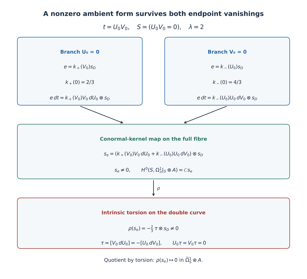
The constructed total space is proper over a disc; it is not asserted to be a compact threefold with vanishing integral first and second cohomology. Thus this example proves the failure of the specified sheaf-level implication, including its extension-to-the-total-space refinement. A conclusion about a compact-threefold theorem requires its additional global hypotheses and its own complete argument.

The exact normalization-kernel calculation in Section 2 and the dimension in (6.4) are taught here from the results recorded in the later review, Section 5, with source labels “prop:kernel” and “prop:sharp.” See the published review source, member s6/paper/s6/s5_correction.tex. These are existing results, independently calculated in this lesson; no priority is claimed.

7. Relative differential forms on the actual total-space charts

The cusp charts in lesson 5 have \(t=xy\) or \(t=xyz\). The finite fillings of lesson 3 have étale covering charts with \(t=s^3\) and \(t=s^4\). We now calculate the ordinary relative differential sheaves on each smooth total-space chart. The base coordinate and the indicated multiplicities remain fixed.

For a holomorphic function \(t\) in \[ R=\mathbb C\{x_1,\ldots,x_n\},\qquad F=\bigoplus_{i=1}^n R\,dx_i, \] the relative module is the cokernel \[ M_t=\Omega^1_{R/\mathbb C\{t\}} =F/R\,dt,\qquad dt=\sum_{i=1}^n (\partial_i t)\,dx_i. \tag{7.1} \] Here \(R\) is the ring of the smooth total space. It has no zero divisors. Torsion in this paragraph means elements killed by a nonzero element of \(R\).

7.1 The exact torsion for a general function

Suppose \(t\) is nonconstant. Choose a greatest common divisor \(\varphi\) of its partial derivatives, keeping its unit ambiguity explicit, and put \[ w=\sum_i\frac{\partial_i t}{\varphi}\,dx_i,\qquad dt=\varphi w. \tag{7.2} \] Division here describes a map into the original module (7.1); it does not replace the original relation \(dt\). The exact result is \[ \operatorname{Tors}M_t=R[w],\qquad R/(\varphi)\longrightarrow R[w],\quad \bar a\longmapsto[a w], \quad\text{an isomorphism}. \tag{7.3} \] Indeed, \(\varphi[w]=[dt]=0\). If \(aw=b\,dt=b\varphi w\), a nonzero component of \(w\) gives \(a=b\varphi\). This proves the stated kernel. Conversely, let a class \([v]\) be killed by \(h\ne0\). Then \(hv=b\varphi w\), so in the fraction field \(v=(b\varphi/h)w\). Write that fraction \(a/c\) with coprime numerator and denominator. Each \(cv_i=aw_i\) forces every prime factor of \(c\) to divide every \(w_i\). The definition of \(\varphi\) excludes such a prime. Hence \(c\) is a unit and \(v\in Rw\). This proves surjectivity. Replacing \(\varphi\) by \(u\varphi\) replaces \(w\) by \(u^{-1}w\); the submodule and the isomorphism with its appropriately changed generator agree.

The ring used here is factorial: the local convergent power-series ring of a smooth complex chart is a regular analytic local ring, and factorization can be proved by induction from Weierstrass preparation and factorization of the associated distinguished polynomial. The argument above uses this factorization only to test divisibility of the displayed coefficients.

At the origin, \(M_t\) is free precisely when \(dt(0)\ne0\). If some partial derivative is a unit, the vector \(dt\) extends to a basis of \(F\), and its quotient is \(R^{n-1}\). If all partials are in the maximal ideal \(\mathfrak m\), then \[ M_t/\mathfrak m M_t\simeq\mathbb C^n, \qquad M_t\otimes_R\operatorname{Frac}(R)\simeq \operatorname{Frac}(R)^{n-1}. \tag{7.4} \] A free module of rank \(n-1\) cannot have the first displayed fibre dimension. This proves the converse.

All factors can also be retained in the normal-crossing expression \[ t=u\,x_1^{m_1}\cdots x_k^{m_k}, \qquad u(0)\ne0,\qquad m_i\ge1. \tag{7.5} \] Write \(x^m=\prod_{i=1}^k x_i^{m_i}\). The full derivatives are \[ \partial_j t= \begin{cases} x^{m-e_j}(x_j\partial_j u+m_j u),&j\le k,\\ x^m\partial_j u,&j>k. \end{cases} \tag{7.6} \] Thus \(\varphi_0=\prod_i x_i^{m_i-1}\) divides every derivative. After that division, the \(j\)-th coefficient for \(j\le k\) is \((\prod_{i\ne j}x_i)(x_j\partial_j u+m_j u)\). The last factor is a unit at the centre. A common prime divisor would have to be one of the \(x_i\), but the coefficient with \(j=i\) is not divisible by it. For \(k=1\) that coefficient is itself a unit. Therefore \(\varphi_0\) is a greatest common divisor up to a unit, with all unit derivatives still present in \(dt/\varphi_0\).

7.2 The double and triple cusp charts

For \(R=\mathbb C\{x,y,z\}\), the two exact presentations are \[ \begin{aligned} M_{xy}&=\frac{R\,dx\oplus R\,dy\oplus R\,dz} {R(y\,dx+x\,dy)},\\ M_{xyz}&=\frac{R\,dx\oplus R\,dy\oplus R\,dz} {R(yz\,dx+xz\,dy+xy\,dz)}. \end{aligned} \tag{7.7} \] Their torsion is zero by (7.3), since the respective coefficient greatest common divisors are units. Their failure of local freeness at a crossing follows from (7.4). The following injective maps prove these conclusions directly and specify their images: \[ \begin{array}{c|ccc|c} &dx&dy&dz&\text{image}\\ \hline M_{xy}\to Re\oplus R\,dz &xe&-ye&dz&(x,y)e\oplus R\,dz\\ M_{xyz}\to Re_1\oplus Re_2 &xe_1&ye_2&-z(e_1+e_2) &Rxe_1+Rye_2+Rz(e_1+e_2). \end{array} \tag{7.8} \] For the first map, a vector \((a,b,c)\) is in the kernel precisely when \(ax=by\) and \(c=0\). Coprimeness of \(x,y\) then gives \((a,b,c)=h(y,x,0)\). For the second, the kernel equations are \(ax=cz\), \(by=cz\). The first forces \(x\mid c\), and the second then forces \(y\mid c/x\). Substitution of \(c=xyh\) gives \((a,b,c)=h(yz,xz,xy)\). In both cases the kernel is exactly the relation in (7.7), proving every assertion in (7.8).

The exact map to the intrinsic sheaf on the full reduced fibre \(S=(t=0)\) is \[ M_t\otimes_R R/(t) =\frac{F}{tF+R\,dt} \xrightarrow{\ \sim\ }\Omega^1_{S/\mathbb C}. \tag{7.9} \] Both sides have the same generators \(dx,dy,dz\) and the same differentiated defining equation. In particular, the torsion-free module \(M_{xy}\) acquires the nonzero class \([y\,dx]=-[x\,dy]\) after this base change. Formula (7.9) is the exact relation between the total-space statement and the fibre calculation in Sections 1–6.

7.3 The two multiple fibres, with their multiplicities

In \(R_m=\mathbb C\{s,y_1,y_2\}\) the original relation is \[ dt=m s^{m-1}\,ds. \] Consequently \[ \begin{aligned} M_{s^3} &=R_3\,dy_1\oplus R_3\,dy_2 \oplus R_3/(3s^2)\,ds,\\ M_{s^4} &=R_4\,dy_1\oplus R_4\,dy_2 \oplus R_4/(4s^3)\,ds. \end{aligned} \tag{7.10} \] The scalar factors \(3\) and \(4\) are units over \(\mathbb C\); hence these ideals are respectively \((s^2)\) and \((s^3)\). The maps identifying the quotient modules keep the class of \(ds\) fixed, and the differentiated relations still have the displayed scalars. Thus the torsion has thickness two at the order-three fibre and thickness three at the order-four fibre.

The quotient actions of lesson 3 are free, so the covering maps from these charts to the fillings are étale. For an étale map \(p:U\to V\) over the base, the differential map is an isomorphism \[ p^*\Omega^1_{V/B}\xrightarrow{\ \sim\ }\Omega^1_{U/B}; \tag{7.11} \] in local holomorphic inverse charts this is the ordinary chain rule. Torsion and local freeness can therefore be read in these charts and descend to the fillings. This argument uses the proved freeness of the actions; no ramified quotient is being substituted for them.

There is also a global formula. For a map whose fibres have the local form (7.5), define the effective divisor \[ Z=\sum_{c\in B} \bigl(f^*(c)-(f^*(c))_{\mathrm{red}}\bigr). \] The saturated image of the original differential map \(df:f^*\omega_B\to\Omega^1_X\) is the line bundle \(f^*\omega_B\otimes\mathcal O_X(Z)\). Indeed, a local frame \(dt/\varphi_0\) maps to the vector obtained from the full coefficients (7.6); (7.3) says that this is precisely the saturation. The quotient of this line by the original \(f^*\omega_B\) is \[ \operatorname{Tors}\Omega^1_{X/B} \simeq \bigl(f^*\omega_B\otimes\mathcal O_X(Z)\bigr)|_Z. \tag{7.12} \] The exact sequence giving the last equality is obtained by tensoring \(0\to\mathcal O_X(-Z)\to\mathcal O_X\to\mathcal O_Z\to0\) with \(f^*\omega_B\otimes\mathcal O_X(Z)\). Under a base change \(t'=\psi(t)\), the differential changes by \(\psi'(t)\); under a change of equation for \(Z\), \(\varphi_0\) changes by its corresponding unit. These are exactly the transitions of the two line bundles, so the local maps glue. In this course’s threefold, \[ Z=2S_1+3S_2. \tag{7.13} \] The reduced cusp contributes zero to (7.13), while its relative one-forms still fail to be locally free at their crossing locus.

7.4 Exterior powers: the double curve reappears

Define \[ \Omega^p_{R/\mathbb C\{t\}} =\frac{\bigwedge^p F}{dt\wedge\bigwedge^{p-1}F} =\bigwedge^p M_t. \tag{7.14} \] The equality follows from the universal property of exterior powers of a quotient. It does not assert preservation of torsion-freeness.

For \(t=xy\), use the ordered basis \((dx\wedge dy,dx\wedge dz,dy\wedge dz)\). The three relation columns \(dt\wedge dx\), \(dt\wedge dy\), \(dt\wedge dz\) are \[ (-x,0,0),\qquad(y,0,0),\qquad(0,y,x). \] Hence \[ \Omega^2_{R/\mathbb C\{xy\}} \simeq R/(x,y)\,(dx\wedge dy) \oplus\frac{R(dx\wedge dz)\oplus R(dy\wedge dz)} {R(y\,dx\wedge dz+x\,dy\wedge dz)}. \tag{7.15} \] The second summand is torsion-free: the proof of (7.3) applies to the primitive vector \((y,x)\). Therefore the first summand is exactly the torsion. It is a nonzero sheaf on the whole double curve.

For \(t=xyz\), wedge product with \(dt\) maps the relative two-forms onto \[ J\,dx\wedge dy\wedge dz,\qquad J=(yz,xz,xy). \] The coefficient map before taking the quotient is \[ (a,b,c)\longmapsto xy\,a-xz\,b+yz\,c. \tag{7.16} \] Its kernel is freely generated by \[ \zeta_1=(z,y,0),\qquad \zeta_3=(0,y,x). \tag{7.17} \] To prove this, (7.16) first gives \(x\mid c\); write \(c=xc'\). Cancellation gives \(y(a+zc')=zb\), so \(z\mid a\); write \(a=za'\). Then \(b=y(a'+c')\), giving precisely \(a'\zeta_1+c'\zeta_3\). Independence follows from their first and third components in the domain \(R\).

In this basis the three original wedge relations are \[ dt\wedge dx=-x\zeta_1,\qquad dt\wedge dy=y(\zeta_1-\zeta_3),\qquad dt\wedge dz=z\zeta_3. \tag{7.18} \] Thus the kernel of the map from relative two-forms onto \(J\) is \[ Q=\frac{R\zeta_1\oplus R\zeta_3} {\langle x\zeta_1,\ y(\zeta_1-\zeta_3),\ z\zeta_3\rangle}. \tag{7.19} \] Each of \(xy,xz,yz\) kills both generators: \(x\zeta_1=0\), \(z\zeta_3=0\), and \(y\zeta_1=y\zeta_3\) give the six products directly. Since \(xy\ne0\) in \(R\), \(Q\) is torsion. The target ideal \(J\subset R\) is torsion-free, so every torsion element of the original relative module is in \(Q\). We have proved \[ \operatorname{Tors}\Omega^2_{R/\mathbb C\{xyz\}}=Q. \tag{7.20} \] Its three relation vectors vanish modulo the maximal ideal, so \(Q/\mathfrak m Q=\mathbb C^2\). It requires two generators, including at the triple point.

The exact homological identification can be checked from the free resolution \[ 0\longrightarrow R^2 \xrightarrow{\left(\begin{smallmatrix}z&0\\y&y\\0&x\end{smallmatrix}\right)} R^3\xrightarrow{(xy,-xz,yz)} R\longrightarrow R/J\longrightarrow0. \tag{7.21} \] The kernel and injectivity were proved in (7.16)–(7.17). Applying \(\operatorname{Hom}_R(-,R)\) gives \[ \operatorname{Ext}^2_R(R/J,R) =R^2/\langle(z,0),(y,y),(0,x)\rangle. \] The coordinate map \((a,b)\mapsto(b,-a)\) carries these generators to \((0,-z),(y,-y),(x,0)\), exactly the relations in (7.19). This proves the claimed isomorphism with \(Q\), including its signs. The space defined by \(J\) is the union of the three coordinate axes. It has dimension one, and \(x+y+z\) is a non-zero-divisor on its ring, since its restriction is nonzero on each axis. Thus it is Cohen–Macaulay; the Ext module in (7.21) is its canonical module.

For \(t=s^m\), keeping the actual derivative yields \[ \Omega^2_{R_m/\mathbb C\{t\}} =R_m\,dy_1\wedge dy_2 \oplus\frac{R_m}{(m s^{m-1})}\,ds\wedge dy_1 \oplus\frac{R_m}{(m s^{m-1})}\,ds\wedge dy_2. \tag{7.22} \] The last two summands are exactly the torsion. Substituting \(m=3\) and \(m=4\) retains the two different scheme thicknesses from (7.10).

For completeness the third exterior power follows from the same relation, without an additional hypothesis: \[ \Omega^3_{R/\mathbb C\{t\}} \simeq \frac{R}{(\partial_x t,\partial_y t,\partial_z t)} \,dx\wedge dy\wedge dz. \tag{7.23} \] Indeed, wedging \(dt\) with each basis two-form generates precisely this coefficient ideal, with the alternating signs absorbed by the indicated generators of the ideal. For \(xy\) this is \(R/(x,y)\); for \(xyz\) it is \(R/(yz,xz,xy)\); and for \(s^m\) it is \(R_m/(m s^{m-1})\) in the coordinate order \((s,y_1,y_2)\). All three are torsion, and all higher exterior powers are zero because \(F\) has rank three.

The one-form calculations and their explicit injections were recorded in the correction note, Proposition 6.1. The general greatest-common-divisor formula, the global divisor (7.12), and the two-form calculations are in the later review, source label “prop:torsion” and the following paragraph. Formula (7.23) is the direct third-exterior-power calculation added here to complete these local presentations. None of these statements alone supplies a direct-image or Hodge-degeneration assertion.

8. Every meromorphic function of the constructed threefold comes from its base

Return to the actual compact threefold \(f:X\to\mathbb P^1\) constructed in lessons 3–5. We use the integral result \(H^2(X;\mathbb Z)=0\) calculated in lesson 7, the compact torus fibres over the regular base locus, and the proved identity \(f_*\mathcal O_X=\mathcal O_{\mathbb P^1}\) from lesson 8. The conclusion is the exact field isomorphism \[ f^*:\mathbb C(\mathbb P^1)\xrightarrow{\ \sim\ }\mathscr M(X), \tag{8.1} \] where \(\mathscr M(X)\) denotes the field of meromorphic functions on \(X\).

First every effective divisor of \(X\) is vertical. Let \(D\) be such a divisor, and suppose one of its irreducible components dominates the base. For a regular fibre \(F\) outside the finitely many fibres contained in \(D\), its restriction \(D|_F\) is then a nonempty effective divisor on the compact complex torus \(F\). A constant positive Hermitian form on the universal covering vector space descends to a Kähler form \(\omega_F\). The cycle class of a divisor is the first Chern class of its divisor line bundle; this follows by the local argument principle applied to transition ratios of its defining functions. Therefore \[ \int_{D|_F}\omega_F =\int_F c_1\!\left(\mathcal O_X(D)|_F\right)\wedge\omega_F. \tag{8.2} \] The left side is strictly positive: the effective cycle has positive integer multiplicities, and the restriction of the positive form has positive area on the smooth locus of each of its curve components. The right side is zero, because \(c_1(\mathcal O_X(D))\) lies in \(H^2(X;\mathbb Z)=0\). This contradiction proves verticality.

There are only finitely many irreducible components of a divisor on compact \(X\). Locally this is the finite factorization of a holomorphic defining equation; a finite covering by such neighbourhoods gives global finiteness. Thus its support is contained in finitely many fibres. Fix a meromorphic function \(h\in\mathscr M(X)\). Its pole divisor is effective, and so has this property.

Choose a base disc \(U\), centred at \(c\), with coordinate \(t\), containing no other pole fibre. Write the full fibre divisor \[ f^*(c)=\sum_i m_i S_i,\qquad m_i\ge1, \] and the pole multiplicities along these components as \(a_i\ge0\). Choose the actual integer \[ N=\max_i\left\lceil\frac{a_i}{m_i}\right\rceil. \tag{8.3} \] Then \((f^*t)^N h\) has no negative divisorial order anywhere on \(f^{-1}(U)\). It is holomorphic: in a smooth local chart write the meromorphic germ as a coprime fraction of convergent power series. A nonunit denominator would have an irreducible factor giving a negative divisorial order. Since none occurs, the denominator is a unit. This also removes any possible indeterminacy in codimension at least two.

The identity \(f_*\mathcal O_X=\mathcal O_{\mathbb P^1}\) now gives a unique holomorphic \(b_U\) on \(U\) such that \[ (f^*t)^N h=f^*b_U,\qquad h=f^*(b_U/t^N). \tag{8.4} \] On discs with no pole fibre we use \(N=0\). On overlaps, the base functions agree because their pullbacks agree and \(f\) is surjective. They therefore glue to a global meromorphic function \(b\) on \(\mathbb P^1\). Conversely, every such \(b\) pulls back meromorphically, and surjectivity of \(f\) also proves injectivity of pullback. This establishes (8.1).

A meromorphic function on \(\mathbb P^1\) is rational: subtract its finitely many principal parts at finite poles; the remainder is entire on \(\mathbb C\) and has at worst a pole at infinity, hence is a polynomial by its power-series coefficients and the Cauchy estimates. Thus \[ \mathscr M(X)=f^*\mathbb C(t),\qquad a(X)=1. \tag{8.5} \] Here algebraic dimension means the transcendence degree of the meromorphic field over \(\mathbb C\). The coordinate \(t\) is transcendental over \(\mathbb C\), since a nonzero constant-coefficient polynomial cannot vanish on its open range; every rational function belongs to \(\mathbb C(t)\). This proves the asserted degree exactly.

The coordinate \(t\) in (8.3) is local at each pole value; its multiplicities include \(3S_1\), \(4S_2\), and the full reduced cusp fibre. No pole is discarded by passing to a reduced divisor. Moreover the fibration recovered from the anticanonical ring in lesson 8 is the same \(f\), up to its proved base automorphism. It therefore realizes the algebraic reduction in (8.1), with the original compact threefold and all its fibres.

9. The entire ambient section space at the actual cusp

Let \(i:W\hookrightarrow X\) be the full reduced cusp fibre over \(p_0\), and let \(\eta:E_0\to W\) be its normalization. Lesson 5 constructs \(E_0=\mathrm{dP}_6\) with its original six rays \[ r_1=(1,0),\ r_2=(0,1),\ r_3=(-1,1),\ r_4=(-1,0),\ r_5=(0,-1),\ r_6=(1,-1). \tag{9.1} \] We will prove that every line bundle \(B\) on \(X\) satisfies \[ \eta^*i^*B\simeq\mathcal O_{E_0},\qquad H^0(W,\widetilde\Omega^1_W\otimes i^*B)=0, \qquad \dim_{\mathbb C}H^0(W,\Omega^1_X|_W\otimes i^*B)=1. \tag{9.2} \] These assertions concern all of \(\operatorname{Pic}(X)\), with no genericity or non-torsion restriction.

9.1 The needed analytic cohomology of the hexagonal surface

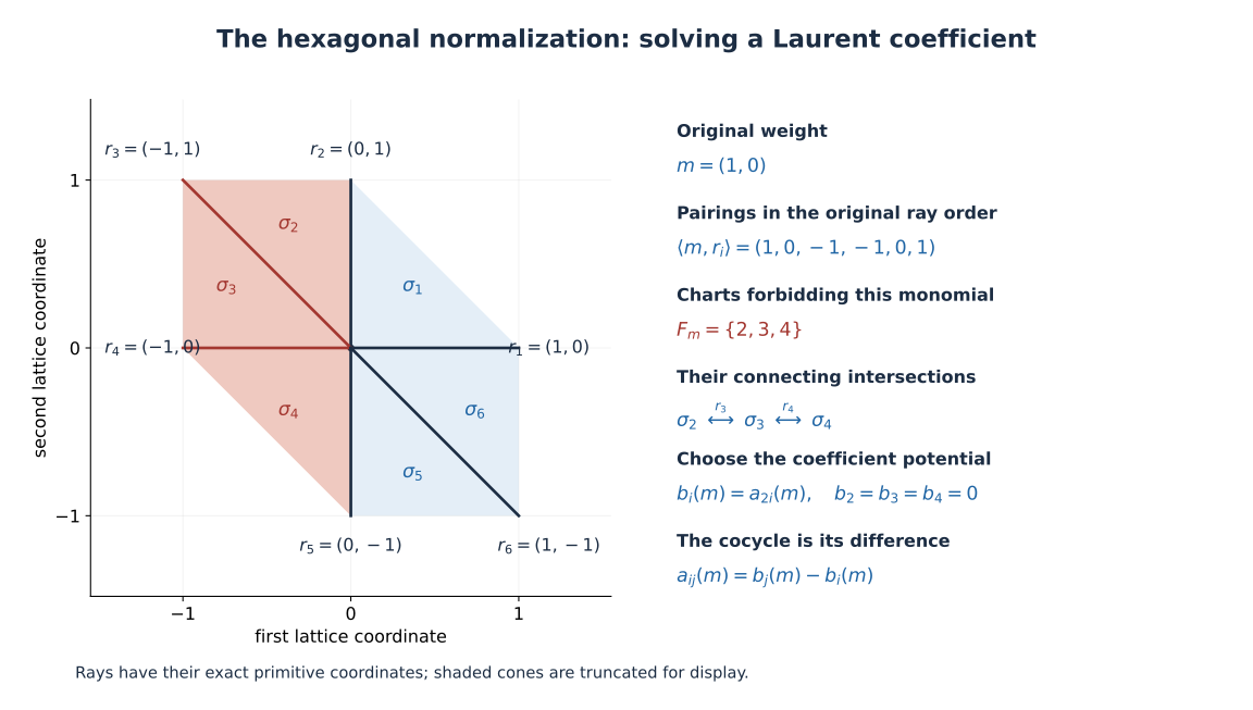
We give the exact vanishing argument \[ H^1(E_0,\mathcal O_{E_0})=0. \tag{9.3} \] Cover \(E_0\) by its six maximal toric charts \(U_i\simeq\mathbb C^2\), for the cones \(\sigma_i=\langle r_i,r_{i+1}\rangle\), with indices modulo six. Every intersection is the chart of the common face: a maximal chart, \(\mathbb C\times\mathbb C^*\), or the dense torus \(T=(\mathbb C^*)^2\). All are Stein. Cartan’s acyclicity theorem therefore makes this cover a Čech cover for \(\mathcal O\).

Let \(g_{ij}\) be an additive holomorphic one-cocycle. Fix the convention \(g_{ij}+g_{jk}=g_{ik}\). On \(T\), expand each function in its unique Laurent series \[ g_{ij}=\sum_{m\in M} a_{ij}(m)\chi^m,\qquad M=\operatorname{Hom}(\mathbb Z^2,\mathbb Z). \tag{9.4} \] Holomorphy on a toric chart containing a ray \(r\) forces \(a_{ij}(m)=0\) if \(\langle m,r\rangle<0\). This is the usual one-variable removable-singularity criterion in the chart coordinate dual to \(r\); the other coordinate is nonzero.

For \(m\ne0\), define \(F_m\) to be the set of chart indices \(i\) for which \(\langle m,r_i\rangle<0\) or \(\langle m,r_{i+1}\rangle<0\). Completeness of the fan implies \(F_m\ne\varnothing\). The rays on which \(m\) is negative lie in a consecutive nonempty block of the cyclic order, since a real linear functional is negative on an open half-plane. Consequently the cones in \(F_m\) are connected by successive intersections whose common ray has negative pairing with \(m\). On every such intersection the coefficient \(a_{ij}(m)\) is zero by the preceding paragraph. The cocycle equation then gives \[ a_{ij}(m)=0\qquad(i,j\in F_m). \tag{9.5} \] Choose one \(j(m)\in F_m\) and set \[ b_i(m)=a_{j(m),i}(m). \tag{9.6} \] For \(m=0\), choose \(j(0)=1\) and use the same formula. Equations (9.5)–(9.6) show that \(b_i(m)=0\) whenever \(m\) is not in the dual cone \(\sigma_i^\vee\). The cocycle equation gives, for every \(m\), \[ b_j(m)-b_i(m)=a_{ij}(m). \tag{9.7} \]

We must check analytic convergence, rather than just formal coefficients. For a fixed \(i\), use the two coordinates of \(U_i\simeq\mathbb C^2\). Every selected coefficient in (9.6) is a coefficient of one of the finitely many functions \(g_{ji}|_T\), expressed in these coordinates. All such Laurent series converge absolutely on every compact product of circles in \(T\). The retained exponents in the coordinates of \(U_i\) are nonnegative. Choose radii \(R_1,R_2\) greater than the coordinate bounds of a given compact polydisc. Cauchy’s coefficient estimate on those circles bounds every selected coefficient by \(C R_1^{-a}R_2^{-b}\), where \(C\) is the maximum of the six circle bounds and \(a,b\ge0\). The two geometric series then prove absolute uniform convergence on the smaller polydisc, including its coordinate axes. Hence \[ b_i=\sum_{m\in\sigma_i^\vee\cap M}b_i(m)\chi^m \] is holomorphic on all of \(U_i\). Formula (9.7) gives \(g_{ij}=b_j-b_i\) on \(T\), and then on the entire overlap by the identity theorem. Every one-cocycle is a coboundary, proving (9.3).

We also need \[ H^0(E_0,\Omega^1_{E_0})=0. \tag{9.8} \] Let \(\pi:E_0\to\mathbb P^2\) be the three point blow-ups explicitly identified in lesson 5. A holomorphic one-form on \(E_0\), restricted off the exceptional curves, gives a one-form on \(\mathbb P^2\) minus the three centres. In an affine coordinate neighbourhood of a centre its two coefficient functions extend across that point by the two-variable removable-singularity theorem. One proof is the Cauchy integral in one variable over a circle avoiding the point, with the other variable free; the identity theorem gives agreement on the punctured neighbourhood. The extended coefficients therefore define a holomorphic one-form on all of \(\mathbb P^2\). Its restriction to every projective line is zero by the proof of (6.2). Every tangent direction at a point of \(\mathbb P^2\) is tangent to one such line, so the form is zero. Its pullback agrees with the original form on a dense open set and hence everywhere. This proves (9.8).

9.2 Pullback of every analytic line bundle

The analytic exponential sequence uses the actual map \(h\mapsto e^{2\pi i h}\): \[ 0\longrightarrow\mathbb Z \longrightarrow\mathcal O_{E_0} \xrightarrow{\,e^{2\pi i(\cdot)}\,}\mathcal O_{E_0}^* \longrightarrow1. \tag{9.9} \] Its long exact sequence and (9.3) show that \[ c_1:\operatorname{Pic}(E_0)\longrightarrow H^2(E_0;\mathbb Z) \quad\text{is injective}. \tag{9.10} \] For a line bundle \(B\) on \(X\), naturality of (9.9) under \(i\circ\eta\) gives \[ c_1(\eta^*i^*B)=(i\circ\eta)^*c_1(B)=0, \tag{9.11} \] because the integral group \(H^2(X;\mathbb Z)\) was calculated to be zero in lesson 7. Injectivity in (9.10) proves the first assertion of (9.2).

This proof uses the already calculated integral cohomology of the same \(X\). The retained source also contains a direct boundary calculation that proves (9.11) without the global Leray transgressions, using the finite-filling norm equations and the cusp support function. Both routes concern the same pullback map in (9.11). The present argument does not assert that a line bundle on a cusp neighbourhood alone has trivial normalized restriction; that stronger local assertion does not follow from (9.11).

The injection from Section 2 gives \[ H^0(W,\widetilde\Omega^1_W\otimes i^*B) \hookrightarrow H^0(E_0,\Omega^1_{E_0}\otimes\eta^*i^*B)=0 \tag{9.12} \] by (9.8) and (9.11). Finally the full kernel isomorphism \(\Phi\), applied to the actual double and triple charts of \(W\), gives \[ \begin{aligned} H^0(W,\Omega^1_X|_W\otimes i^*B) &\simeq H^0(E_0,\eta^*(N^*_{W/X}\otimes i^*B))\\ &\simeq H^0(E_0,\mathcal O_{E_0})\otimes T_{p_0}^*B_{\mathrm{base}}. \end{aligned} \tag{9.13} \] In the last term \(B_{\mathrm{base}}=\mathbb P^1\); this notation distinguishes the base curve from the line bundle \(B\). The last isomorphism chooses a nonzero frame of \(\eta^*i^*B\); the first is canonical. Since \(E_0\) is connected and compact, its holomorphic functions are constant. The right side is one-dimensional. This completes the proof of (9.2).

9.3 The conormal factor and adjunction cancel exactly

It is useful to keep the one-dimensional base factors visible. Intrinsically, \[ N^*_{W/X}\simeq\mathcal O_W\otimes T_{p_0}^*B_{\mathrm{base}}, \qquad \mathcal O_X(W)|_W\simeq \mathcal O_W\otimes T_{p_0}B_{\mathrm{base}}. \tag{9.14} \] The first map sends a cotangent vector \(dt|_{p_0}\) to the class \([f^*t]\) in \(I_W/I_W^2\). A coordinate change \(t'=\psi(t)\) multiplies this generator by \(\psi'(0)\); the second map transforms by its inverse. For the dualizing line of the Cartier fibre, adjunction is \[ \omega_W=\omega_X|_W\otimes\mathcal O_X(W)|_W. \tag{9.15} \] Given any \(L\in\operatorname{Pic}(X)\), set \(A=L^\vee|_W\otimes\omega_W\). Equations (9.14)–(9.15) give the canonical equality of line bundles \[ N^*_{W/X}\otimes A \simeq (L^\vee\otimes\omega_X)|_W. \tag{9.16} \] The twist \(A\) is the restriction of the actual global line bundle \(L^\vee\otimes\omega_X\otimes\mathcal O_X(W)\). Thus (9.12) applies to it. The canonical first isomorphism in (9.13), before choosing any frame, now yields \[ H^0(W,\Omega^1_X|_W\otimes L^\vee|_W\otimes\omega_W) \simeq H^0(E_0,\eta^*(L^\vee\otimes\omega_X)|_W) \simeq\mathbb C. \tag{9.17} \] The first displayed map includes the exact cancellation of the tangent and cotangent factors. Only the final identification with \(\mathbb C\) chooses a frame. Formula (9.17) computes the entire space entering duality.

10. Cartier duality and the exact top-degree fibre map

We now pass from the explicitly computed ambient cotangent sections to the tangent-bundle cohomology. The divisor in this argument is the full scheme-theoretic fibre, including its multiplicities whenever the argument is applied at one of the two finite fillings.

10.1 The duality map for a Cartier divisor

Let \(j:S\hookrightarrow Y\) be an effective Cartier divisor in a compact smooth complex threefold, and let \(E\) be a holomorphic vector bundle on \(Y\). The divisor may be non-normal, reducible, or nonreduced. Its two-term vector-bundle resolution is \[ 0\longrightarrow E\otimes\mathcal O_Y(-S) \xrightarrow{\,\iota\,}E \longrightarrow j_*(E|_S)\longrightarrow0. \tag{10.1} \] In a local divisor equation \(g\), the first map is multiplication by \(g\). It is injective because \(g\) is a non-zero-divisor and \(E\) is locally free.

The smooth Serre trace is the integration pairing \[ H^q(Y,V)\times H^{3-q}(Y,V^\vee\otimes\omega_Y) \longrightarrow\mathbb C,\qquad ([\alpha],[\beta])\longmapsto\int_Y\operatorname{ev}(\alpha\wedge\beta). \tag{10.2} \] Dolbeault representatives give the displayed \((3,3)\)-form. The included smooth duality provider, Sections1–4, proves the local resolution, weak elliptic estimates, compact resolvent and harmonic contraction, and constructs the perfect pairing (10.2). It embeds a canonical-line-valued form with its antiholomorphic factor before its canonical form. In that exact order its integration-by-parts sign is \((-1)^{q+1}\), and its conjugate-linear metric map has the full phase \((-1)^{n(n-1)/2}i^{-n}\). These formulas prove nondegeneracy on the actual finite-dimensional harmonic representatives. They require a Hermitian metric and ellipticity, with no Kähler assumption.

Apply this trace to the two vector bundles in (10.1). More explicitly, put them in degrees \(-1,0\) and take their Dolbeault resolutions. Totalization gives a complex computing \(R\Gamma(S,E|_S)\). The evaluation pairing (10.2), applied to each term with the total-complex signs, gives a map from its dual total complex to the dual of its cohomology complex. On either single vector-bundle term it is a quasi-isomorphism by (10.2). The two-step filtration of the total complex then proves that it is a quasi-isomorphism for (10.1) as well. This constructs the duality map, rather than inferring a pairing just from matching dimensions.

The sheaf dual of (10.1), before the dimension-three shift, is \[ E^\vee\otimes\omega_Y \xrightarrow{\,\iota^\vee\,} E^\vee\otimes\omega_Y\otimes\mathcal O_Y(S) \tag{10.3} \] in degrees \(0,1\). Locally the map again multiplies by \(g\). Its kernel is zero and its cokernel is \[ j_*\bigl(E^\vee|_S\otimes (\omega_Y\otimes\mathcal O_Y(S))|_S\bigr). \tag{10.4} \] The full line-bundle transition from a change \(g'=ug\) is included in \(\mathcal O_Y(S)\). Thus (10.4) identifies the dualizing line \[ \omega_S=(\omega_Y\otimes\mathcal O_Y(S))|_S \tag{10.5} \] and locates it in Ext degree one. The shift by three in (10.2), followed by this Ext degree one, gives the exact degree-two formula \[ H^q(S,E|_S)^\vee \xrightarrow{\ \sim\ } H^{2-q}(S,E^\vee|_S\otimes\omega_S). \tag{10.6} \] There is no negative coherent cohomology, so (10.6) also proves \(H^q(S,E|_S)=0\) for \(q>2\). All the maps are natural in \(E\), because they come from evaluation and precomposition in the dual complex. Nothing in (10.1)–(10.6) used normality or reducedness.

10.2 Flatness over the actual base curve

For the constructed \(f:X\to\mathbb P^1\), fix \(x\in X\), write \(c=f(x)\), and put \[ A=\mathcal O_{\mathbb P^1,c},\qquad R=\mathcal O_{X,x}. \] The map \(A\to R\) is injective. If a nonzero one-variable holomorphic germ composed with \(f\) were zero near \(x\), then \(f\) would have image in its discrete zero set and would be locally constant. The identity theorem on connected \(X\) would make \(f\) constant everywhere, contrary to the constructed fibration.

The ring \(A\) is a discrete valuation ring, and \(R\) is a domain. Thus \(R\) is torsion-free as an \(A\)-module. Such a module is flat: every finitely generated submodule is a finitely generated torsion-free module over the principal ideal domain \(A\), hence free by successive division by a uniformizer; the whole module is the filtered union of these free submodules. Tensor product commutes with that filtered union, and filtered unions preserve exact sequences of modules, which proves flatness. The same holds for each locally free \(R\)-module. Consequently \(f\) is flat and every vector bundle \(E\) on \(X\) is \(f\)-flat.

If \(t\) is a base uniformizer, \(f^*t\ne0\) in the domain \(R\). Every full fibre is therefore a Cartier divisor. In the finite charts these are exactly \((s^3)\) and \((s^4)\); in the cusp charts they are \((xy)\) or \((xyz)\). Compactness of \(X\) makes \(f\) proper.

10.3 Why the degree-two map is an isomorphism

The included graph-resolution provider, Sections1–5, constructs the required analytic finite complex for this actual compact smooth total space and vector bundle. It resolves the graph in \(X\times U\) by its full Cartier ideal, including the local equations \(s^3-\tau\), \(s^4-\tau\), \(xy-\tau\), and \(xyz-\tau\). Its explicit smooth bundle comparison is holomorphic in \(\tau\). The resulting two-term Dolbeault cone has the proved compact Hodge contraction, and the full perturbation formulas give a finite holomorphic complex with actual inclusion, projection and chain homotopy. The parameter Cauchy argument in its Section5 proves that this complex represents the direct image and that evaluation gives the canonical fibre map. Thus, on a sufficiently small neighbourhood of \(c\), there is a bounded complex \(K^\bullet\) of finite free base modules representing \(Rf_*E\), with \[ H^q(K^\bullet\otimes_A\mathbb C(c)) \simeq H^q(X_c,E|_{X_c}). \tag{10.7} \] Here the fibre in the right side has its full scheme structure. Flatness proved above, and the injectivity of the restricted graph equation, identify its ordinary restriction with the derived restriction. The provider’s Section6 also proves coherence by finite matrices over the convergent one-variable local ring. This establishes the exact finite-complex form of analytic cohomology and base change used here; the individual direct images may have torsion.

We spell out the exact algebra that this theorem supplies in the present problem. Since every term of \(K^\bullet\) is free, multiplication by the uniformizer gives a short exact sequence of complexes \[ 0\longrightarrow K^\bullet \xrightarrow{\,t\,}K^\bullet \longrightarrow K^\bullet\otimes_A\mathbb C(c) \longrightarrow0. \] Its cohomology sequence gives \[ 0\longrightarrow H^q(K^\bullet)/tH^q(K^\bullet) \longrightarrow H^q(K^\bullet\otimes_A\mathbb C(c)) \longrightarrow H^{q+1}(K^\bullet)[t]\longrightarrow0. \tag{10.8} \] The notation \(M[t]\) means the kernel of multiplication by \(t\) on \(M\). The two-term free resolution \(A\xrightarrow{t}A\) of \(\mathbb C(c)\) identifies it with \(\operatorname{Tor}_1^A(M,\mathbb C(c))\). Thus (10.8) retains exactly the possible obstruction to base change.

For \(q>2\), the middle term is zero by (10.6) applied to the compact Cartier fibre \(X_c\subset X\). Therefore the first term is zero. The finite generation of \(H^q(K^\bullet)\), followed by Nakayama’s lemma, gives \(H^q(K^\bullet)=0\). This works at every \(c\), so \[ R^q f_*E=0\qquad(q>2). \tag{10.9} \] At \(q=2\) the last term in (10.8) is consequently zero. The remaining map is precisely the canonical fibre map, and we obtain \[ \beta_c^2: (R^2f_*E)_c\otimes_A\mathbb C(c) \xrightarrow{\ \sim\ }H^2(X_c,E|_{X_c}). \tag{10.10} \] This proof neither assumes constancy of \(h^2\) nor concludes that \(R^2f_*E\) is locally free. For example, over \(A=\mathbb C\{t\}\) the free complex \(A\xrightarrow{t}A\) in degrees \(1,2\) has \(H^2=A/(t)\), which is not free, and the degree-two fibre map is nevertheless an isomorphism. Its fibre dimension jumps from zero away from \(0\) to one at \(0\).

The general proper-flat surface theorem proves the same top-degree conclusion without smoothness or compactness of the total space. It includes the full analytic construction and compact coherent dimension bound. The preceding graph and Cartier-duality proof remains the direct route for this course’s actual threefold.

10.4 The result for every tangent-bundle twist

Take \(E=T_X\otimes L\), where \(L\) is any analytic line bundle on the original \(X\). At the actual cusp \(W\), (10.6) and (9.17) give \[ \begin{aligned} H^2(W,(T_X\otimes L)|_W)^\vee &\simeq H^0(W,\Omega^1_X|_W\otimes L^\vee|_W\otimes\omega_W)\\ &\simeq H^0(E_0,\eta^*(L^\vee\otimes\omega_X)|_W). \end{aligned} \tag{10.11} \] The last line has dimension one by the calculation in Section 9. Therefore \[ \boxed{\ \dim_{\mathbb C}H^2(W,(T_X\otimes L)|_W)=1,\qquad \dim_{\mathbb C} \bigl((R^2f_*(T_X\otimes L))_{p_0}\otimes\mathbb C(p_0)\bigr)=1 \ }\quad(L\in\operatorname{Pic}(X)). \tag{10.12} \] The second equality is (10.10), with exactly the same bundle and full fibre. In particular \(R^2f_*(T_X\otimes L)\ne0\) for every \(L\). Its stalk at \(p_0\) is a nonzero finite module with one-dimensional residue fibre. Nakayama’s lemma says that it needs exactly one local generator; it does not determine the annihilator or its length, and those are not asserted in (10.12).

The conormal calculation, the base tangent-line cancellation, the trace, and the fibre map in (10.11)–(10.12) explain the complete route from the original cusp geometry to the direct-image failure. The retained reconstruction supplies the same duality and base-change route in the source labels “thm:cartier-duality,” “cor:surface-top-base-change,” and “cor:candidate-conductor-actual.” The refinement from nonzero to dimension one uses the normalization-kernel result already recorded in the later review and proved in Section 2 here.

11. The full index polynomial and global nonvanishing

For this compact complex threefold and every analytic line bundle \(L\), we will obtain \[ \chi(X,T_X\otimes L)=1,\qquad H^2(X,T_X\otimes L)\ne0. \tag{11.1} \] The first equality is an analytic index calculation. The second also uses the effective fibre divisor and the holomorphic family of all line bundles; the Euler characteristic alone does not determine each cohomology group.

11.1 The analytic index and the complex orientation

For a holomorphic vector bundle \(V\) on a compact complex manifold \(Y\), choose Hermitian metrics and use the Dolbeault operator with its adjoint, \[ D_V=\sqrt2\,(\bar\partial_V+\bar\partial_V^*): \mathcal A^{0,\mathrm{even}}(Y,V) \longrightarrow\mathcal A^{0,\mathrm{odd}}(Y,V). \tag{11.2} \] Let \(\mathscr D_V=\sqrt2(\bar\partial_V+\bar\partial_V^*)\) act on all form degrees. Then \(D_V\) in (11.2) is its even-to-odd restriction and \(D_V^*\) is its odd-to-even restriction. The included Hodge proof, Section3, retains the exact factor and proves \[ \mathscr D_V^2=2\bigl(\bar\partial_V\bar\partial_V^* +\bar\partial_V^*\bar\partial_V\bigr). \] Thus the kernels of \(D_V\) and \(D_V^*\) are precisely the even and odd harmonic Dolbeault forms. The analytic index is therefore exactly \(\sum_q(-1)^q h^q(Y,V)\). The included tangent-index proof constructs this operator’s integer homomorphism on smooth bundle classes, proves its exact invariance under torsion line-bundle twists, and transfers the full de Rham differential to the finite Dolbeault harmonic complex. In complex dimension three, smooth Serre duality and the actual contraction map \(T_Y\otimes K_Y\to\Omega_Y^2\) then prove \[ \chi(Y,T_Y\otimes L)=\frac12\chi_{\mathrm{top}}(Y) \] whenever \(c_1(K_Y)\) and \(c_1(L)\) are torsion as integral classes. Its diagonal Thom calculation identifies the right side with \(\langle c_3(T_Y),[Y]\rangle/2\). These are complete receiving proofs for the original threefold and for the further generality in Section11.5. The full characteristic factors and their exact polynomial comparison follow.

If \(x_1,\ldots,x_n\) denote the formal Chern roots of \(T^{1,0}Y\), the full characteristic factor is \[ e^{c_1(TY)/2}\,\widehat A(TY_{\mathbb R}) = e^{(\sum_i x_i)/2} \prod_i\frac{x_i/2}{\sinh(x_i/2)} =\prod_i\frac{x_i}{1-e^{-x_i}} =\operatorname{td}(TY). \tag{11.3} \] The middle equality follows separately for every root from \(2\sinh(x/2)=e^{x/2}-e^{-x/2}\); all exponential factors remain in the comparison. Characteristic identities in these formal roots descend by the splitting principle. The orientation is the complex orientation \((e_1,Je_1,\ldots,e_n,Je_n)\). For a compact complex threefold \(Y\) with torsion \(c_1(K_Y)\) and \(c_1(L)\), the receiving proof gives \[ \chi(Y,T_Y\otimes L) =\left\langle\operatorname{ch}(T_Y)\operatorname{ch}(L) \operatorname{td}(TY),[Y]\right\rangle. \tag{11.4} \] Indeed its Section6 computes the complete polynomial below, proves the vanishing of each contribution involving those two torsion first classes, and identifies the remaining \(c_3/2\) evaluation with the independently computed analytic index. This establishes (11.4) under its exact stated hypotheses, including all Picard components when \(b_2=0\). The broader human reference is Paul Baum and Erik van Erp, arXiv:1604.03502v1, Theorem1 and its appendix on complex Spin\({}^c\) structures. The receiving proof here is complete without assuming that paper’s general index theorem.

11.2 Every term of the tangent-bundle polynomial

Put \(c_i=c_i(T_X)\) and \(\ell=c_1(L)\), with cohomological degrees \(2i\) and \(2\). Up to degree six the factors in (11.4) are exactly \[ \begin{aligned} \operatorname{ch}(T_X) &=3+c_1+\tfrac12(c_1^2-2c_2) +\tfrac16(c_1^3-3c_1c_2+3c_3),\\ \operatorname{ch}(L) &=1+\ell+\tfrac12\ell^2+\tfrac16\ell^3,\\ \operatorname{td}(T_X) &=1+\tfrac12c_1+\tfrac1{12}(c_1^2+c_2) +\tfrac1{24}c_1c_2. \end{aligned} \tag{11.5} \] These formulas follow by expanding \(\sum_i e^{x_i}\), \(e^\ell\), and \(\prod_i x_i/(1-e^{-x_i})\), then using the elementary symmetric expressions for \(c_1,c_2,c_3\). Higher-degree terms have zero pairing with the six-dimensional fundamental class; no such term contributes to (11.4).

Multiplying the displayed factors, before applying any topological vanishing, gives the complete degree-six expression \[ \begin{aligned} \bigl[\operatorname{ch}(T_X)\operatorname{ch}(L) \operatorname{td}(T_X)\bigr]_6 ={}&\frac12c_3+\frac12c_1^3-\frac{19}{24}c_1c_2\\ &+\frac54\ell c_1^2-\frac34\ell c_2 +\frac54\ell^2c_1+\frac12\ell^3. \end{aligned} \tag{11.6} \] For example, the coefficient of \(c_1c_2\) is the sum \[ \frac3{24}+\frac1{12}-\frac12-\frac12=-\frac{19}{24}; \] these four terms come respectively from tangent Chern-character degrees \(0,2,4,6\). The coefficient of \(\ell c_1^2\) is \(3/12+1/2+1/2=5/4\), that of \(\ell c_2\) is \(3/12-1=-3/4\), and that of \(\ell^2c_1\) is \(3/4+1/2=5/4\). The rank-three term gives \(\ell^3/2\). This checks every mixed contribution.

The integral calculation in lesson 7, Sections 1–8, gives \(H^2(X;\mathbb Z)=H^4(X;\mathbb Z)=0\). Hence \(c_1,\ell\) and \(c_2\) vanish in these actual cohomology groups; every term in (11.6) other than \(c_3/2\) therefore pairs to zero for this stated reason. The included index provider, Section6, proves the complete Thom and signed-diagonal comparison: the top Chern class is the Euler class in complex orientation, the diagonal normal map is \(v\mapsto(-v,v)\) with determinant \(2^6>0\), and its full dual-basis formula evaluates to the alternating sum of Betti numbers. The integral ranks calculated in lesson7 make this value \(1+1=2\). Thus (11.4)–(11.6) give \[ \chi(X,T_X\otimes L) =\frac12\langle c_3(T_X),[X]\rangle =\frac12\cdot2=1 \tag{11.7} \] for every \(L\). In particular this value does not depend on a choice of period parameter.

11.3 Generic endpoint vanishing, with the actual family

Let \(D=f^*(c)\) be any nonzero full fibre divisor. For any vector bundle \(V\) on compact connected \(X\), view \[ V_m=H^0(X,V\otimes\mathcal O_X(-mD)) \quad\text{as a subspace of }H^0(X,V). \] These are decreasing finite-dimensional vector spaces, so their dimensions eventually stop decreasing, and the spaces themselves then stabilize. An element of the stable value vanishes to order at least \(m\) along \(D\) for every \(m\). At a point of \(D\), write its coefficients in a local frame and let \(g\) be the local defining function of \(D\). Divisibility by every \(g^m\), whose orders tend to infinity, makes every Taylor coefficient zero. The section vanishes on a neighbourhood of that point and therefore on all of connected \(X\). We have proved \[ H^0(X,V(-mD))=0\quad\text{for all sufficiently large }m. \tag{11.8} \] This proof applies to the actual multiplicities of \(D\); it uses its defining function, without replacing it by a reduced equation.

The exponential sequence on \(X\), together with \(H^1(X;\mathbb Z)=H^2(X;\mathbb Z)=0\), gives \[ \operatorname{Pic}(X)\simeq H^1(X,\mathcal O_X)\simeq\mathbb C^q. \tag{11.9} \] To realize this as a holomorphic family, take additive Čech representatives \(a_{ij}^{(r)}\) of a basis of \(H^1(X,\mathcal O_X)\). On the product with \(\mathbb C^q\), the transition functions \[ \exp\!\left(2\pi i\sum_{r=1}^q z_r a_{ij}^{(r)}\right) \tag{11.10} \] satisfy the multiplicative cocycle condition. They define a line bundle whose restriction at \(z\) is the class in (11.9). Thus all twists in the argument below belong to one specified holomorphic family.

For this exact family, the included finite-complex construction, Sections5–6, provides actual finite matrices of holomorphic functions computing its cohomology. It starts from the operator \(\bar\partial_V+2\pi i\sum_r z_r b_r\wedge(-)\), constructs its frames with exactly the transitions (11.10), and proves all inclusion, projection and contraction identities. The factor \(2\pi i\) and the parameter coordinates \(z_r\) are unchanged. Consequently the loci \(h^k\ge1\) are closed analytic: if the vector space in degree \(k\) has rank \(n_k\), then \[ h^k=n_k-\operatorname{rank}(d_{k-1}) -\operatorname{rank}(d_k). \] The inequality \(h^k\ge1\) is a finite union of simultaneous rank bounds, each imposed by vanishing minors of matrices of holomorphic functions. These local loci agree on intersections and hence give a closed analytic subset. A proper analytic subset of the connected vector space \(\mathbb C^q\) has dense open complement.

Apply (11.8) first to \(V=T_X\). It supplies one twist with \(H^0=0\), so degree-zero vanishing holds on a dense open subset of (11.9). Apply it next to \(V=\Omega^1_X\otimes\omega_X\). Smooth Serre duality (10.2) gives \[ H^3(X,T_X\otimes\mathcal O_X(\ell D))^\vee \simeq H^0(X,\Omega^1_X\otimes\omega_X(-\ell D))=0 \tag{11.11} \] for sufficiently large positive \(\ell\). Therefore degree-three vanishing also holds on a dense open subset. Their intersection \(U\) is dense open, and \[ h^0(X,T_X\otimes L)=h^3(X,T_X\otimes L)=0 \qquad(L\in U). \tag{11.12} \]

11.4 Nonvanishing for every line bundle

For \(L\in U\), equations (11.7) and (11.12) yield the exact equality \[ h^2(X,T_X\otimes L) =1+h^1(X,T_X\otimes L)\ge1. \tag{11.13} \] The locus \(h^2\ge1\) is closed and contains the dense subset \(U\). It is therefore all of \(\operatorname{Pic}(X)\). We have proved the second part of (11.1), including twists outside \(U\). Formula (11.13) does not assert that the global group always has dimension one; (10.12) is the separate exact dimension calculation on the cusp fibre.

There is a useful consequence for any surjective holomorphic map \(g:X\to C\) to a smooth compact curve: \[ R^2g_*(T_X\otimes L)\ne0 \qquad\text{for every }L. \tag{11.14} \] Here is the full implication. Suppose this direct image were zero, and write \(E=T_X\otimes L\). Fix a point \(c\in C\). For a coherent sheaf \(Q\) on \(C\), \[ H^1(C,Q(mc))=0\qquad(m\gg0). \tag{11.15} \] To prove (11.15), its torsion subsheaf has finite support and no positive cohomology, and the quotient is a vector bundle because the local curve rings are discrete valuation rings. For that vector bundle, curve Serre duality identifies \(H^1(Q(mc))^\vee\) with \(H^0(Q^\vee\otimes\omega_C(-mc))\). The decreasing-section proof of (11.8), applied at the point \(c\), makes this zero for large \(m\). The torsion exact sequence proves the assertion for \(Q\).

Use (11.15) for \(Q=R^1g_*E\). Projection formula, the assumed \(R^2g_*E=0\), and the fact that a curve has no coherent cohomology above degree one make every Leray term of total degree two for \(E\otimes g^*\mathcal O_C(mc)\) zero: \[ H^2(C,g_*E\otimes\mathcal O_C(mc))=0,\quad H^1(C,R^1g_*E\otimes\mathcal O_C(mc))=0,\quad H^0(C,R^2g_*E\otimes\mathcal O_C(mc))=0. \] Consequently \(H^2(X,E\otimes g^*\mathcal O_C(mc))=0\), contradicting the already proved nonvanishing for every line-bundle twist. This proves (11.14).

11.5 The further generality already present in the review

The same complete argument proves the following statement. If \(Y\) is any compact connected complex threefold with \[ b_1(Y)=b_2(Y)=b_3(Y)=0 \] and a nonzero effective divisor, then \(H^2(Y,T_Y\otimes L)\ne0\) for every analytic line bundle \(L\), and \(R^2g_*(T_Y\otimes L)\ne0\) for every holomorphic map onto a smooth compact curve.

We check the changes to the proof. The groups \(H^1(Y;\mathbb Z)\) and \(H^2(Y;\mathbb Z)\) are respectively zero and finite: the first is the torsion-free dual of \(H_1\), and the second is finitely generated of rank zero by the universal coefficient theorem. Thus \(\operatorname{Pic}^0(Y)\simeq H^1(Y,\mathcal O_Y)\), and every component of \(\operatorname{Pic}(Y)\) is its translate. The class of the divisor line bundle is torsion; choose its finite order \(r\). The divisor \(rD\) is still nonzero and effective, and its line bundle is in \(\operatorname{Pic}^0(Y)\). On a fixed component \(L_0\operatorname{Pic}^0(Y)\), apply (11.8) to \(T_Y\otimes L_0\) and to its Serre-dual bundle, using \(rD\). The explicit family (11.10), tensored with \(L_0\), proves the two dense open endpoint vanishings in that component.

Rationally, \(c_1(TY)\), \(c_1(L)\), and \(c_2(TY)\) vanish because \(H^2(Y;\mathbb Q)=H^4(Y;\mathbb Q)=0\), the latter by Poincaré duality. All terms in (11.6) except \(c_3/2\) therefore vanish after pairing. Poincaré duality and the three stated Betti numbers give \(\chi_{\mathrm{top}}(Y)=2\), so (11.7) still gives \(1\). Closedness of the degree-two jump locus proves nonvanishing on each component separately. The proof of (11.14) then applies verbatim with \(Y\).

More generally, if only \(b_1=b_2=0\), the same evaluation is \[ \chi(Y,T_Y\otimes L)=1-\frac12 b_3(Y). \tag{11.16} \] The cup-product pairing on \(H^3(Y;\mathbb Q)\) is nondegenerate and skew-symmetric, so \(b_3\) is even. To see the parity, a nonzero alternating form admits a pair with nonzero pairing; their two-dimensional span is nondegenerate, and splitting off that span inductively leaves a sum of such pairs. If a degree-two group vanished at one twist, its vanishing locus in that component would be dense open. Intersecting with the two endpoint open sets would give \(\chi=-h^1\le0\), and hence \(b_3\ge2\) by (11.16). This proves the surviving global implication and all its hypotheses. The nonvanishing theorem above is its application when \(b_3=0\).

These strengthenings to Betti-number hypotheses, all Picard components, and an arbitrary nonzero effective divisor were already proved in the later review, Section 5 under “What survives: the derived global criterion.” The source correction note states the more restricted algebraic-reduction version. The calculations here teach the stronger result with its complete receiving argument and retain the full polynomial (11.6).

12. The exact comparison with the 1998 and 2020 statements

The preceding proofs identify three different mathematical issues: a split group extension still retains its monodromy in abelianization; a singular fibre retains its intrinsic cotangent torsion in the conormal sequence; and the compact threefold has a positive tangent-bundle index. We give the precise maps and source locations for each.

12.1 Abelianization of the actual split extension

Choose a splitting of a group extension and write \(G=K\rtimes Q\). Its abelianization is \[ G^{\mathrm{ab}}\simeq (K^{\mathrm{ab}})_Q\oplus Q^{\mathrm{ab}}, \qquad (K^{\mathrm{ab}})_Q =K^{\mathrm{ab}}/\langle q\cdot[k]-[k]\rangle. \tag{12.1} \] The map sends \((k,q)\) to \(([k],[q])\). It is a homomorphism because in the coinvariant quotient \([q\cdot k']=[k']\); hence the semidirect product law maps to addition. It is onto. Its kernel is generated by commutators inside \(K\), commutators inside \(Q\), and the cross-commutators \(qkq^{-1}k^{-1}\). All these vanish in every abelian quotient, while quotienting by all of them makes the displayed target abelian. Thus its kernel is exactly \([G,G]\), proving (12.1) and its inverse universal property.

For example, \[ G=\mathbb Z\rtimes_{-1}\mathbb Z =\langle a,t\mid tat^{-1}=a^{-1}\rangle \] has a splitting \(n\mapsto t^n\), but abelianization makes its single relation \(2[a]=0\), so \[ G^{\mathrm{ab}}=\mathbb Z[t]\oplus(\mathbb Z/2)[a]. \tag{12.2} \] The projection to each factor and the defining presentation prove that no additional relation occurs.

For our middle family, lesson 6 proves \[ \pi_1(X^\circ)=\Lambda\rtimes F(\rho_1,\rho_2) \] with the original integral matrices \(A_1,A_2\). Use the lattice basis \((\widehat\gamma,\widehat u,\widehat w,\widehat\delta)\) dual to the original cohomology marking. The first rows of \(A_j-I\) are zero, so all monodromy relations lie in \(\langle\widehat u,\widehat w,\widehat\delta\rangle\). Three actual relation columns are \[ a=(A_1-I)\widehat w=\widehat u-2\widehat w,\qquad b=(A_2-I)\widehat u=-\widehat u+\widehat w,\qquad c=(A_1-I)\widehat u=-\widehat u-\widehat w+\widehat\delta. \] They generate that entire rank-three sublattice, since \[ \widehat u=-a-2b,\qquad \widehat w=-a-b,\qquad \widehat\delta=c-2a-3b. \tag{12.3} \] Consequently the exact integral quotient and abelianization are \[ \Lambda_{\langle A_1,A_2\rangle}=\mathbb Z[\widehat\gamma], \qquad H_1(X^\circ;\mathbb Z) =\mathbb Z[\widehat\gamma]\oplus \mathbb Z[\rho_1]\oplus\mathbb Z[\rho_2]. \tag{12.4} \] In particular its rank is three. A direct sum retaining all of \(H_1(F;\mathbb Z)=\Lambda\) would instead have rank six.

Dualizing the actual restriction map gives \[ \operatorname{im}\bigl(H^1(X^\circ;\mathbb Z) \longrightarrow H^1(F;\mathbb Z)\bigr) =\mathbb Z\gamma =H^1(F;\mathbb Z)^{\langle T_1,T_2\rangle}. \tag{12.5} \] Indeed, every character of the semidirect product restricts to an invariant character of \(\Lambda\), and every invariant character extends by setting its two base-generator values to zero. Thus (12.5) proves both inclusions and gives an explicit extension.

The map from this subgroup to \(H^1(F,\mathcal O_F)\) is also exact in the original periods. Write the fibre coordinates as \(\zeta_1,\zeta_2\), and retain \[ \Pi= \begin{pmatrix}6\mu&\tau&1&0\\ \beta&\mu&0&1\end{pmatrix}, \quad T=\operatorname{Im}\tau,\quad m=\operatorname{Im}\mu,\quad b_0=\operatorname{Im}\beta,\quad a_0=\frac mT,\quad D=b_0-\frac{6m^2}{T}<0. \] The imaginary parts of the two coordinate differentials give \[ \gamma= \frac{d\zeta_2-a_0d\zeta_1 -d\bar\zeta_2+a_0d\bar\zeta_1}{2iD}. \] Projection to Dolbeault degree \((0,1)\), the map induced by the inclusion of constant functions into holomorphic functions, therefore sends \[ \gamma\longmapsto \frac{a_0\,d\bar\zeta_1-d\bar\zeta_2}{2iD}. \tag{12.6} \] This class is nonzero. Integration of a derivative of a periodic function over the torus has mean zero, so it cannot equal this nonzero constant coefficient. Fourier expansion also shows that every \(\bar\partial\)-closed \((0,1)\)-form has, modulo a \(\bar\partial\)-derivative, a unique constant representative: for each nonzero real frequency the symbol is wedge product by a nonzero \((0,1)\)-covector, whose Koszul complex is exact by contraction with a dual vector. Its norm is bounded below by a positive constant times the real frequency norm, since the fixed real-to-\((0,1)\) map is an isomorphism of real vector spaces. The resulting division has polynomial bounds in frequency and preserves the rapid decay of smooth Fourier coefficients. Thus \(H^1(F,\mathcal O_F)\) has the basis \(d\bar\zeta_1,d\bar\zeta_2\).

The complex span of the image in (12.6) is therefore exactly a one-dimensional subspace of this two-dimensional space. This computes the specific integral-to-holomorphic map used by the printed rank argument. It does not infer a restriction on every holomorphic section of a direct-image bundle merely from monodromy; (12.5)–(12.6) specify the domain to which the calculation applies.

In the original-author TeX of Campana–Demailly–Peternell, arXiv:math/9607215, the split-extension inference appears in Lemma 5.2(2), followed by the spanning argument in the proof of Theorem 5.1. The published numbering cited in the later reconstruction is Lemma 3.2 and Theorem 3.1. The 2020 original-author TeX repeats the direct-sum inference in Lemma 4.2. Equations (12.1) and (12.4) give its replacement and the actual value for this family. The correction retains the projection to the base, the original monodromy, and the full integral fibre lattice.

12.2 The conormal inference at the non-normal fibre

At the start of Section 7 of the 2020 original-author TeX, source label “eq:main1” (published page 692), the conormal sequence is used to reduce ambient vanishing to \[ H^0(S,\widetilde\Omega^1_S\otimes A)=0 \] when the line-bundle restriction is non-torsion. Sections 1–3 of this lesson compute the exact intermediate sheaf \(\mathscr K_S\). If both that displayed group and \(H^0(S,N^*_{S/X}\otimes A)\) vanish, the actual ambient group is \[ \ker\!\left( H^0(S,\mathscr T_S\otimes A) \xrightarrow{\delta_A} H^1(S,N^*_{S/X}\otimes A)\right). \tag{12.7} \] The proper nodal family of Sections 4–6 has both endpoint vanishings and a nonzero kernel, even with the explicit infinite-order twist extending to its smooth total space. This proves failure of the indicated inference.

The actual cusp \(W\) supplies the global application: (9.17) and (10.12) compute the full Serre-dual space and prove that the degree-two fibre group has dimension one for every global twist. These statements use the constructed compact \(X\) and its established Picard pullback. Thus the global comparison does not rely on treating the disc test family as a compact example.

12.3 Which theorem conclusions the constructed \(X\) contradicts

The hypotheses in the 2020 Theorem 2.2, source label “MT2,” are all verified for this same object:

• \(X\) is a connected compact smooth complex threefold, by the complete finite and cusp gluing in lessons 3–5.
• \(H^1(X;\mathbb Z)=H^2(X;\mathbb Z)=0\), by the integral calculation of lesson 7.
• \(a(X)=1\), and its algebraic reduction is the holomorphic \(f:X\to\mathbb P^1\), by Section 8 here.

The theorem asserts tangent-twist vanishing in degrees other than one, nonpositive tangent-twist Euler characteristic, and nonpositive top Chern number. Equations (11.1) and (11.7) instead give, for every twist, \[ H^2(X,T_X\otimes L)\ne0,\qquad \chi(X,T_X\otimes L)=1,\qquad \langle c_3(T_X),[X]\rangle=2. \tag{12.8} \] Thus each of these three conclusions fails for the constructed threefold, including any generic-twist interpretation of the first conclusion.

The earlier 1998 Theorem 4.1 states constancy of all meromorphic functions for a compact complex threefold with \(b_2=0\) and nonzero \(c_3\). Its two hypotheses hold here, whereas \(f\) supplies a nonconstant meromorphic function and (8.1) computes the whole field. The sphere statements in 1998 Corollary 4.2 and 2020 Corollary 2.3 assert algebraic dimension zero. Their additional hypothesis is an actual homeomorphism to \(S^6\), the recognition question treated in lesson 7. Integral cohomology and Euler characteristic alone do not supply that identification. The compact-threefold comparison (12.8) uses the hypotheses itemized above.

The 2020 Theorem 2.1, source label “MT1,” has a different additional hypothesis: a nonconstant meromorphic map to \(\mathbb P^1\) that does not extend holomorphically. It is absent here. By (8.1), every meromorphic map to \(\mathbb P^1\) is a rational function of \(f\). A rational function of the coordinate on \(\mathbb P^1\) defines a holomorphic self-map of \(\mathbb P^1\): take its coprime numerator and denominator and homogenize both to the larger degree. There is no common finite zero, and at infinity at least one leading coefficient is nonzero. They therefore give a well-defined holomorphic map in homogeneous coordinates. Composing with \(f\) gives a holomorphic map on \(X\). Consequently this construction supplies no counterexample to Theorem 2.1 or to the alternative proof of that case cited there by Lehn–Rollenske–Schinko.

The source originals are Campana–Demailly–Peternell, arXiv:math/9607215 and their corrigendum, arXiv:1904.11179v2. The statements above were compared with their original-author TeX. The later correction and review sources are linked in Sections 5–7; their historical narrow scope for the disc test family is preserved in Section 6, while the actual compact-object calculation supplies the stronger conclusion in (12.8).

13. Four worked exercises

Exercise 1. Extend every gluing scalar

For the same proper cubic family (4.1), prove that every \(A_\lambda\), \(\lambda\in\mathbb C^*\), extends to a line bundle on the total family after possibly shrinking its base disc. Give the extending divisor, cover the exceptional values of your parameter formula, and compute the ambient section-space dimension even when \(\lambda=1\).

Solution. Keep the section \(P(t)\) from (5.4), with \(P(0)\) corresponding to \(a=0\). For \(\lambda\ne-1\), put \[ b=\frac{\lambda-1}{\lambda+1}. \tag{13.1} \] It is never \(1\), since \(\lambda-1=\lambda+1\) is impossible, and it is never \(-1\), since that would give \(\lambda=0\). If also \(\lambda\ne1\), then \(b\ne0\), and the central smooth point \[ Q_b(0)=[b^2-1:b(b^2-1):1] \] has nonzero second coordinate. It extends by the explicit holomorphic section \[ Q_b(t)= \left[b^2-1: \sqrt{\,b^2(b^2-1)^2+t\,}:1\right], \tag{13.2} \] where the square root has value \(b(b^2-1)\) at \(0\). A sufficient square-root domain is \(|t|<|b^2(b^2-1)^2|/2\), further intersected with the original disc and the domain of \(P(t)\). Direct substitution into (4.1) verifies the section. The central points are distinct, so after a further shrink the two sections are disjoint. The relative divisor line bundle \[ \mathcal O_{\mathscr C}(P-Q_b) \] has, by (5.8), scalar \[ \frac{1+b}{1-b}=\lambda. \tag{13.3} \] If \(\lambda=1\), use the trivial bundle on \(\mathscr C\). If \(\lambda=-1\), take \(Q_\infty(t)=[0:1:0]\) and use \(\mathcal O_{\mathscr C}(P-Q_\infty)\). On the normalization its divisor is \([0]-[\infty]\), so a nowhere-zero frame is \(s_{P-Q_\infty}/r\). The ratio of its coefficient at \(q=-1\) to the coefficient at \(p=1\) is \(-1\), as required.

These cases exhaust \(\mathbb C^*\). Taking the product pullback extends the bundle to \(\mathcal X\). The radius is allowed to depend on \(\lambda\); the calculation has not asserted a common radius for all unbounded scalars and both exceptional limits.

For every \(\lambda\), the normalized pullback is trivial and \(H^0(\mathbb P^1\times\mathbb P^1,\Omega^1)=0\). Section 3 therefore computes \[ H^0(S,\Omega^1_{\mathcal X}|_S\otimes \operatorname{pr}_1^*A_\lambda)\simeq\mathbb C. \tag{13.4} \] When \(\lambda=1\), the generator is the original ambient \(dt|_S\). In this case \(H^0(S,A_\lambda)=\mathbb C\), so the first endpoint vanishing is absent; the dimension formula itself remains valid. For \(\lambda\ne1\) both endpoints vanish. The bundle is of infinite order precisely when \(\lambda\) is not a root of unity, by the exact tensor-power rule \(A_\lambda^{\otimes n}=A_{\lambda^n}\).

This proves the stronger extension statement for every scalar, beyond the single extending scalar explicitly displayed in the correction note. The result concerns the same proper local family and retains its prescribed central gluing convention.

Exercise 2. Determine the exact annihilator at a triple point

For the module \(Q\) in (7.19), prove \[ \operatorname{Ann}_R(Q)=(xy,xz,yz). \tag{13.5} \] Describe its restriction at the generic point of each coordinate axis and its fibre at the triple point.

Solution. Equations (7.18)–(7.20) show that the ideal \(J=(xy,xz,yz)\) kills both generators of \(Q\), so \(J\subset\operatorname{Ann}_R(Q)\). Localize at the prime \((y,z)\), corresponding to the \(x\)-axis. The element \(x\) is a unit, so \(\zeta_1=0\). The two remaining relations are \(y\zeta_3=z\zeta_3=0\). Hence \[ Q_{(y,z)}\simeq R_{(y,z)}/(y,z)\cdot\zeta_3. \] At \((x,z)\), \(y\) is a unit and \(\zeta_1=\zeta_3\); the result is \[ Q_{(x,z)}\simeq R_{(x,z)}/(x,z)\cdot\zeta_1. \] At \((x,y)\), \(z\) is a unit and \(\zeta_3=0\); the result is \[ Q_{(x,y)}\simeq R_{(x,y)}/(x,y)\cdot\zeta_1. \tag{13.6} \] Each is one-dimensional over the fraction field of its axis. If a germ annihilates \(Q\), (13.6) forces it to lie in each of the three primes, and \[ (y,z)\cap(x,z)\cap(x,y)=(xy,xz,yz). \] To verify this intersection directly, expand a convergent series into monomials. Restriction to all three axes vanishes exactly when each nonzero monomial contains at least two distinct variables. Assign each such monomial to one of \(xy,xz,yz\) dividing it; the three corresponding subseries remain convergent on smaller polydiscs. This expresses the germ in \(J\). Therefore the reverse inclusion in (13.5) holds.

At the origin, all three relation vectors in (7.19) have coefficients in the maximal ideal, so \(Q/\mathfrak m Q=\mathbb C^2\). Thus the module is generically of rank one on each of the three axes and needs two generators at their meeting point. Its support and annihilator are exactly those of the reduced three-axis curve, not a thickening inferred only from a schematic picture.

Exercise 3. What does a one-dimensional direct-image fibre determine?

Let \[ M=(R^2f_*(T_X\otimes L))_{p_0}, \qquad A=\mathcal O_{\mathbb P^1,p_0}\simeq\mathbb C\{t\}. \] Use (10.12) to classify the possible \(A\)-module \(M\). State exactly which information remains undetermined by the residue-fibre calculation.

Solution. Coherence makes \(M\) a finite \(A\)-module, and (10.12) gives \(\dim_{\mathbb C}M/tM=1\). Lift a nonzero residue class to \(m\in M\). The quotient \(M/Am\) has zero residue quotient, so Nakayama’s lemma makes it zero. Thus \(A\to M\), \(a\mapsto am\), is onto. Its kernel is an ideal of the discrete valuation ring \(A\), hence either \(0\) or \((t^r)\) for \(r\ge0\). The case \(r=0\) would make \(M=0\), contradicting its residue dimension. Therefore \[ M\simeq A\quad\text{or}\quad M\simeq A/(t^r)\ (r\ge1). \tag{13.7} \] In the first case the stalk is free of rank one. In the second it is torsion of length \(r\). All these possibilities have the same one-dimensional residue fibre. This proves why neither local freeness nor a torsion length can be read from (10.12) alone. Formula (13.7) is the complete classification that the exact dimension and coherence provide.

Exercise 4. Retain the third Betti number in the global calculation

Let \(Y\) be a compact connected complex threefold with \(b_1=b_2=0\) and a nonzero effective divisor. On each Picard component, determine the exact relation between \(h^1\) and \(h^2\) on the dense open set where \(h^0=h^3=0\). Determine what a single vanishing \(H^2(Y,T_Y\otimes L)=0\) forces.

Solution. Retain the entire index polynomial (11.6). The degree-two and degree-four rational groups vanish, so the only nonzero possible pairing is \(c_3/2\). Poincaré duality gives \[ \langle c_3(T_Y),[Y]\rangle =1-b_1+b_2-b_3+b_4-b_5+1=2-b_3. \] Section 11.5 supplies the simultaneous endpoint vanishing in each Picard component, including the torsion class of its initial bundle. On that dense open set, \[ h^2(Y,T_Y\otimes L) =h^1(Y,T_Y\otimes L)+1-\frac{b_3}{2}. \tag{13.8} \] The alternating nondegenerate middle pairing makes \(b_3=2k\) for an integer \(k\ge0\). For \(k=0\), (13.8) forces \(h^2\ge1\), and closedness of the jump locus extends nonvanishing to the whole component. For \(k=1\), it gives \(h^2=h^1\), so the numerical argument allows both to vanish. For \(k>1\), it gives \(h^1=h^2+k-1\ge k-1\).

If \(H^2\) vanishes at one point, its vanishing is a nonempty analytic open set and hence dense in that component. Intersect it with the endpoint open set. There (13.8) becomes \(h^1=k-1\ge0\), so \(k\ge1\), equivalently \(b_3\ge2\). This proves the exact surviving implication without introducing an unproved vanishing for the original threefold.

14. Line-bundle factors and the three boundary equations

The preceding cohomological proof of the cusp restriction uses the integral calculation of lesson 7. There is also a direct route through the actual line-bundle factors of the three fillings. We give that route because it explains how the two finite fillings constrain a line bundle near the non-normal fibre. Its source is the retained programme argument, Analytic completion of the all-Picard certificate, Proposition “analytic Appell–Humbert boundary cocycle” and Theorem “purely analytic vanishing of the global restriction.” The following proof keeps the covering spaces, the original period matrix, and the signs of the clockwise meridians explicit.

Write \[ \Lambda=\mathbb Z\widehat\gamma\oplus\mathbb Z\widehat u \oplus\mathbb Z\widehat w\oplus\mathbb Z\widehat\delta, \qquad V=\operatorname{Hom}(\Lambda,\mathbb Z) =\mathbb Z\gamma\oplus\mathbb Zu\oplus\mathbb Zw\oplus\mathbb Z\delta. \] The hat distinguishes a vector from its dual covector. Products of covectors below are exterior products. The original homology matrices \(A_1,A_2\) of lesson 6 induce the following contragredient matrices on \(V\): \[ T_1=(A_1^{-1})^{\mathsf t} =\begin{pmatrix} 1&0&-6&2\\0&-1&1&1\\0&-1&0&1\\0&0&0&1 \end{pmatrix}, \qquad T_2=(A_2^{-1})^{\mathsf t} =\begin{pmatrix} 1&6&0&-3\\0&0&-1&1\\0&1&0&0\\0&0&0&1 \end{pmatrix}. \tag{14.1} \] For all \(g\) and \(\lambda\), \[ \langle T_g\alpha,\lambda\rangle =\langle\alpha,A_g^{-1}\lambda\rangle. \tag{14.2} \] In particular these matrices must not be interchanged with \(A_1,A_2\).

14.1. The invariant two-form and the integral coinvariants

Let \(L\) be an arbitrary holomorphic line bundle on the actual compact threefold. On a smooth fibre \(F\), the exponential connecting class is an alternating integral form \[ E=c_1(L|_F)\in\bigwedge\nolimits^2V. \] Transporting the same bundle around the two base loops preserves this form. We compute its possible values without using the global cohomology of \(X\).

Put \[ E=a\gamma u+b\gamma w+c\gamma\delta +d\,uw+e\,u\delta+f\,w\delta. \] In this ordered basis, the coefficient vectors of \((\bigwedge^2T_1-I)E\) and \((\bigwedge^2T_2-I)E\) are respectively \[ \begin{pmatrix} -2a+b+c-6d+2e-8f\\ -a-b+c-6d+2e-6f\\ -6f\\f\\-2e+f\\-e-f \end{pmatrix}, \qquad \begin{pmatrix} -a-b+c-6d+6e-3f\\ a-b+3e\\ 6e\\-e\\-e-f\\e-f \end{pmatrix}. \tag{14.3} \] These expressions come from applying each matrix to each of the two covectors in every exterior product. The fourth entries give \(f=e=0\). The second entry of the second column then gives \(a=b\); subtracting the first two entries of the first column gives \(-a+2b=0\). Thus \(a=b=0\), and either first entry gives \(c=6d\). Conversely substitution verifies all twelve equations. Therefore, over the integers, \[ E=kq,\qquad k\in\mathbb Z,\qquad q=uw+6\gamma\delta. \tag{14.4} \]

We also need the quotient \[ V_G=V/\bigl((T_1-I)V+(T_2-I)V\bigr). \] Every relation has zero \(\delta\)-coefficient. Define the actual relation vectors \[ \begin{aligned} a_1&=(T_1-I)u=-2u-w,& a_2&=(T_2-I)w=-u-w,\\ a_3&=(T_1-I)\delta=2\gamma+u+w,& a_4&=(T_2-I)\delta=-3\gamma+u. \end{aligned} \] Then \[ u=a_2-a_1,\qquad w=a_1-2a_2,\qquad \gamma=-a_1-a_3-a_4. \tag{14.5} \] All three equalities are integral. They prove both the quotient and its lack of hidden torsion: \[ V_G=\mathbb Z[\delta]. \tag{14.6} \] In particular the quotient map is exactly evaluation on \(\widehat\delta\).

14.2. The original factors determine a real crossed homomorphism

Take a small open Riemann-surface neighbourhood \(P^{\mathrm{an}}\) of the pair-of-pants core in the punctured base. Its universal cover is contractible and Stein. The fibre vector cover is \[ \widetilde{\mathcal J}=\widetilde P^{\mathrm{an}}\times\mathbb C^2, \] with fibre translation \(\tau_\lambda(z,\zeta)=(z,\zeta+\Pi(z)\lambda)\), where \(\Pi\) is the full original period matrix. The exponential sequence and Cartan’s theorem B trivialize the pullback of \(L\) to this contractible Stein manifold.

Choose a frame. For a deck transformation \(\alpha\), define its factor \(a_\alpha\) by the convention \[ a_{\alpha\beta}(x)=a_\alpha(\beta x)a_\beta(x). \] Every factor has a holomorphic logarithm, because this covering space is simply connected: \[ a_\alpha=e^{2\pi i h_\alpha},\qquad c(\alpha,\beta) =h_\alpha(\beta x)+h_\beta(x)-h_{\alpha\beta}(x)\in\mathbb Z. \tag{14.7} \] The integer is independent of \(x\). Expanding the two ways of multiplying three factors proves the two-cocycle identity. Thus the pairs \((r,\alpha)\), \(r\in\mathbb R\), with product \[ (r,\alpha)(s,\beta) =(r+s+c(\alpha,\beta),\alpha\beta) \tag{14.8} \] form the pushout to \(\mathbb R\) of the integral central extension. Denote its central element \((r,1)\) by \(\mathbf c(r)\). The original integers, factors and logarithms remain (14.7); passage to (14.8) is a specified inclusion of their central coefficient group.

On the translation subgroup the commutator integer is \[ c(\tau_\lambda,\tau_\mu)-c(\tau_\mu,\tau_\lambda) =E(\lambda,\mu). \tag{14.9} \] To check its sign, follow the four oriented sides \(\lambda,\mu,-\lambda,-\mu\) of the period parallelogram. The changes of logarithm of the transition units telescope to the difference on the left. Dividing their winding by \(2\pi i\) is the exponential connecting class evaluated on that ordered parallelogram. This is our convention for \(E\).

Choose auxiliary lifts \(U_\lambda\) of \(\tau_\lambda\) with \[ U_\lambda U_\mu =\mathbf c\!\left(\frac12E(\lambda,\mu)\right)U_{\lambda+\mu}. \tag{14.10} \] Here is the precise comparison with the original cocycle, including the correction it requires. Restrict \(c\) to translations and subtract \(E/2\); the resulting real cocycle has zero alternating part. Its extension is therefore abelian. Lift an integral basis of the free abelian group \(\Lambda\) to that abelian extension and multiply the lifts to obtain a splitting. Equivalently there is a real function \(b:\Lambda\to\mathbb R\) such that \[ c(\tau_\lambda,\tau_\mu) +b(\lambda)+b(\mu)-b(\lambda+\mu) =\frac12E(\lambda,\mu). \] Multiplying each original translation lift by \(\mathbf c(b(\lambda))\) gives (14.10). Thus no factor in (14.7) has been discarded. Two such auxiliary systems differ by \[ U'_\lambda=\mathbf c(\langle a,\lambda\rangle)U_\lambda \quad\text{for a unique }a\in V_{\mathbb R}. \tag{14.11} \] Indeed, their central ratio is additive by (14.10).

Let \(\widehat g\) be the zero-section lift of a base deck transformation. Original period equivariance gives \[ \widehat g\,\tau_\lambda\,\widehat g^{-1}=\tau_{A_g\lambda}. \] Choose an extension lift \(G_g\), and define \(d(g)\) by \[ G_gU_{A_g^{-1}\lambda}G_g^{-1} =\mathbf c(\langle d(g),\lambda\rangle)U_\lambda. \tag{14.12} \] Conjugation preserves (14.9), so \(E(A_g\lambda,A_g\mu)=E(\lambda,\mu)\). Applying this identity to (14.10) proves that the exponent in (14.12) is additive in \(\lambda\); it therefore defines an element of \(V_{\mathbb R}\). Applying (14.12) successively to \(h\) and \(g\) gives \[ \begin{aligned} \langle d(gh),\lambda\rangle &=\langle d(g),\lambda\rangle +\langle d(h),A_g^{-1}\lambda\rangle,\\ d(gh)&=d(g)+T_gd(h). \end{aligned} \tag{14.13} \] The lift of \(gh\) may differ centrally from \(G_gG_h\); the difference cancels under conjugation. Replacing the translation lifts as in (14.11) changes \[ d(g)\longmapsto d(g)+(T_g-I)a. \tag{14.14} \] A central change of \(G_g\) has no effect.

Retain the based clockwise loops and the zero-section whiskers of lesson 6. Their actual relation is \[ \rho_1\rho_2\rho_0=1,\qquad \widehat\rho_1\widehat\rho_2\widehat\rho_0=1, \] with no terminal fibre translation. Writing \(d_i=d(\rho_i)\), (14.13) gives \[ d_1+T_1d_2+T_1T_2d_0=0,\qquad \bar d_1+\bar d_2+\bar d_0=0 \quad\text{in }V_G\otimes\mathbb R. \tag{14.15} \]

14.3. The finite fillings give the full norm equations

For filling \(j\), let \[ \widetilde J_j=\Delta_j\times\mathbb C^2,\qquad r_j:\widetilde J_j\to J'_j \] be the vector cover and the lattice quotient. Keep the two vector-cover transformations from lesson 3: \[ \begin{aligned} Q_{j,\log}\tau_\lambda Q_{j,\log}^{-1} &=\tau_{A_j\lambda},& Q_{j,\log}^{m_j}&=\tau_{v_j},\\ Q_{j,\mathrm{lin}}\tau_\lambda Q_{j,\mathrm{lin}}^{-1} &=\tau_{A_j\lambda},& Q_{j,\mathrm{lin}}^{m_j}&=1, \end{aligned} \tag{14.16} \] where \[ (m_1,m_2)=(3,4),\qquad v_1=(1,2,-4,0)^{\mathsf t},\qquad v_2=(-1,-3,3,0)^{\mathsf t}. \] The sign \(+v_j\) comes from \(m_j\) clockwise iterations with \(s_j\mapsto e^{-2\pi i/m_j}s_j\). The descended transformations \(q_{j,\log},q_{j,\mathrm{lin}}\) on \(J'_j\) both have order \(m_j\), since the fibre translation in (14.16) becomes the identity there.

On \(J_j^{\prime *}\), the actual translation \(h_j\) constructed in lesson 3 satisfies \[ h_jq_{j,\log}h_j^{-1}=q_{j,\mathrm{lin}}. \] With quotient maps \[ p_{j,\log}:J_j^{\prime *}\to N_j^*,\qquad p_{j,\mathrm{lin}}:J_j^{\prime *}\to J_j^*, \] it induces \(\bar h_j:N_j^*\to J_j^*\), and \[ p_{j,\mathrm{lin}}h_j=\bar h_jp_{j,\log}. \] Consequently the gluing of the line bundle is the exactly typed isomorphism \[ p_{j,\log}^*(L|_{N_j^*}) \simeq h_j^*p_{j,\mathrm{lin}}^*(L|_{J_j^*}). \tag{14.17} \]

For the following comparison, the punctured vector cover is not simply connected. We therefore compare factors on its universal cover, and retain the map to the full filled vector cover. This makes the relation between the two deck groups explicit. The boundary group is \[ \Gamma_{\partial j} =\Lambda\rtimes_{A_j}\mathbb Z =\langle\tau_\lambda,\rho_j: \rho_j\tau_\lambda\rho_j^{-1}=\tau_{A_j\lambda}\rangle. \] The filled deck group is \[ \Gamma_j =\langle\tau_\lambda,Q_{j,\log}: Q_{j,\log}\tau_\lambda Q_{j,\log}^{-1}=\tau_{A_j\lambda}, \ Q_{j,\log}^{m_j}=\tau_{v_j}\rangle. \] The inclusion of the punctured filling induces the homomorphism \[ \varphi_j:\Gamma_{\partial j}\to\Gamma_j,\qquad \tau_\lambda\mapsto\tau_\lambda,\quad \rho_j\mapsto Q_{j,\log}. \tag{14.18} \] To verify the second image without an unrecorded translation, lift the clockwise zero-section path first through \(p_{j,\mathrm{lin}}\), then through \(h_j^{-1}\), and finally through \(r_j\). The first endpoint is \(q_{j,\mathrm{lin}}h_j(x)\), the second is \(q_{j,\log}x\), and the last is \(Q_{j,\log}\widetilde x\). In the last step use the same branches as lesson 3, \(\ell'(w)=\ell(g_j^{-1}w)-2\pi i/m_j\). Their exact translation difference is the one already contained in \(Q_{j,\log}\); it adds neither \(\tau_\lambda\) nor an inverse generator. The fixed whisker identifies this boundary path with the globally based \(\rho_j\). Fibre loops remain \(\tau_\lambda\) because \(h_j\) is a fibre translation.

The pullback of \(L|_{N_j}\) to \(\widetilde J_j\) is trivial. Its factors and their logarithms give a central extension of \(\Gamma_j\), by (14.7)–(14.8). Pull this extension back by \(\varphi_j\). On the universal cover of the punctured vector cover, (14.17) identifies it with the global boundary extension. To verify this assertion directly, let the ratio of the two pulled-back frames be \(F=e^{2\pi i H}\), which has a logarithm on this simply connected space. The two factor logarithms then differ by \(H(\alpha x)-H(x)\) and an integer depending on \(\alpha\). Substitution into (14.7) cancels the terms involving \(H\), leaving the coboundary of that integer. Thus the two central extensions are isomorphic, with the identity on the central group. This proves the comparison on the correct deck group \(\Gamma_{\partial j}\); it does not identify that group with its quotient \(\Gamma_j\).

Construct \(\widetilde d_j:\Gamma_j\to V_{\mathbb R}\) from the filled extension by (14.12). The same multiplication calculation proves \[ \widetilde d_j(\alpha\beta) =\widetilde d_j(\alpha)+T_\alpha\widetilde d_j(\beta). \] The comparison just proved, together with (14.11), gives a character \(a_j\in V_{\mathbb R}\) with \[ \widetilde d_j(Q_{j,\log}) =d_j+(T_j-I)a_j. \tag{14.19} \] For a fibre translation choose its lift to be \(U_v^{(j)}\). Its commutator with \(U_\lambda^{(j)}\) is \(\mathbf c(E(v,\lambda))\), so \[ \widetilde d_j(\tau_v)=\iota_vE,\qquad (\iota_vE)(\lambda)=E(v,\lambda). \] Apply the crossed law to the full relation (14.16). Since \(T_j^{m_j}=I\), the term involving \(a_j\) cancels exactly: \[ \begin{aligned} N_{T_j}d_j &=N_{T_j}\widetilde d_j(Q_{j,\log})\\ &=\widetilde d_j(Q_{j,\log}^{m_j}) =\widetilde d_j(\tau_{v_j}) =\iota_{v_j}E, \qquad N_{T_j}=\sum_{r=0}^{m_j-1}T_j^r. \end{aligned} \tag{14.20} \] A branch change \(\ell\mapsto\ell+2\pi i n\) changes the vector lift of the comparison by \(\tau_{nv_j}\). Conjugation by \(U_{nv_j}\) changes the comparison character by \(n\iota_{v_j}E\). But \[ T_j(\iota_{v_j}E)(\lambda) =E(v_j,A_j^{-1}\lambda) =E(A_jv_j,\lambda)=E(v_j,\lambda), \] using the original invariant vector \(A_jv_j=v_j\). Thus this branch change leaves (14.19) and (14.20) unchanged. Central changes of extension lifts also cancel. These computations prove the full norm equations with their signs and their choice-independence.

14.4. The cusp gives its remaining coordinate

The original cusp monodromy fixes \(\widehat\delta\). Equation (14.12) therefore reads \[ [G_0,U_{\widehat\delta}] =\mathbf c(\langle d_0,\widehat\delta\rangle). \tag{14.21} \] The exponent is the logarithmic clutching winding with the base loop first. In the actual unimodular cusp chart use \[ (u,x_1,x_2),\qquad t_c=ux_1x_2, \] and the torus \[ (\theta,\phi)\longmapsto \bigl(\rho e^{i(\theta-\phi)},1,e^{i\phi}\bigr), \qquad t_c=\rho e^{i\theta}. \tag{14.22} \] Here increasing \(\phi\) at fixed \(\theta\) is the fibre loop \(\widehat\delta\). Put \(\alpha=\theta-\phi\). In the coordinates consisting of the \(u\)-longitude \(a_u\) and the \(x_2\)-meridian \(m_{x_2}\), \[ b=a_u,\qquad f=m_{x_2}-a_u,\qquad b\wedge f=a_u\wedge m_{x_2}. \tag{14.23} \] The determinant is \(+1\). In particular the fixed-base fibre loop itself is not the boundary of the disc with \(u\) fixed; (14.23) is the comparison that justifies use of that disc.

Choose an annulus \(A_u\) about \(|u|=\rho\), a disc \(D_1\) about \(1\), and a disc \(D_2\) containing \(|x_2|\le1\), with \[ A_u\times D_1\times D_2\subset\{|ux_1x_2|<\epsilon\}. \] This is possible by first choosing bounded discs and then taking \(\rho\) small. The product is Stein and retracts to a circle. Hence its second integral cohomology is zero; Cartan’s theorem B and the exponential sequence give zero Picard group. The pulled-back bundle has one holomorphic frame on this entire product. In that frame the transition across a cut of the \(u\)-longitude is \(1\), with meridian winding \[ \frac1{2\pi i}\int_{|x_2|=1}\frac{d1}{1}=0. \] By (14.23), this is the base-first winding in (14.21). Its value is unchanged by a frame change: in the deck group the elements \(\widehat\rho_0,\tau_{\widehat\delta}\) commute, so the alternating part of any group coboundary on that pair is zero. Thus \[ \langle d_0,\widehat\delta\rangle=0,\qquad \bar d_0=0\quad\text{in }V_G\otimes\mathbb R. \tag{14.24} \] Using fibre-first orientation would insert a minus sign in the winding comparison; the resulting zero is the same. Equation (14.23) records that sign choice explicitly.

14.5. All three fillings force the fibre Chern form to vanish

Keep the integral covectors \[ \eta_1=2u+w+3\delta,\qquad \eta_2=u+w+2\delta. \] Direct contraction of the full \(q=uw+6\gamma\delta\) with the original vectors gives \[ \iota_{v_1}q=4u+2w+6\delta=2\eta_1,\qquad \iota_{v_2}q=-3u-3w-6\delta=-3\eta_2. \tag{14.25} \] Equation (14.6) gives \([\eta_1]=3[\delta]\) and \([\eta_2]=2[\delta]\). Apply the coinvariant quotient to (14.20), retaining both orders: \[ 3\bar d_1=6k[\delta],\qquad 4\bar d_2=-6k[\delta]. \] Consequently \[ \bar d_1=2k[\delta],\qquad \bar d_2=-\frac32k[\delta],\qquad 0=\bar d_1+\bar d_2+\bar d_0=\frac{k}{2}[\delta]. \tag{14.26} \] The last group is \(\mathbb R[\delta]\), so \(k=0\). We have proved \[ c_1(L|_F)=E=0\qquad\text{for every }L\in\operatorname{Pic}(X) \tag{14.27} \] from the line-bundle factors of the three fillings. The cusp equation alone would give only (14.24); the incompatible nonzero contributions in (14.26) are what force (14.27).

15. Recovering the central restriction from the original toric family

Vanishing of the form on a nearby fibre does not, by itself, identify a line bundle on the normalization of the central fibre. We now construct and prove the exact comparison for the cusp of lesson 5. This is the second part of the retained source’s analytic argument, Lemma “the toric support function detects central restriction.”

Let \(M\in\operatorname{Pic}(N_0)\), let \(\pi:Y_\epsilon\to N_0\) be the actual cusp covering, and set \(\mathcal M=\pi^*M\). The deck maps are the original maps \[ \Psi_\lambda(x,t_c) =\bigl(t_c^{B_0\lambda}c_\lambda(t_c)x,t_c\bigr), \quad B_0=\begin{pmatrix}0&1\\-1&0\end{pmatrix}, \quad c_\lambda(t_c)=\exp(2\pi iC(t_c)\lambda), \tag{15.1} \] where \[ C(t_c)= \begin{pmatrix}6\mu(t_c)&h(t_c)\\b(t_c)-h(t_c)&\mu(t_c)\end{pmatrix}, \qquad Z=sB_0+C(t_c),\quad e^{2\pi is}=t_c. \] All entries and all units in this formula are retained. The equality \(\pi\Psi_\lambda=\pi\) supplies genuine descent maps \(\theta^\mathcal M_\lambda:\Psi_\lambda^*\mathcal M\to\mathcal M\) with their cocycle identity.

The toric boundary components are \(E_v\), \(v\in\mathbb Z^2\). The map \(\Psi_\lambda\) sends \(E_v\) to \(E_{v+B_0\lambda}\). At \(E_0\), order the six boundary directions as \[ r_1=(1,0),\ r_2=(0,1),\ r_3=(-1,1),\ r_4=(-1,0),\ r_5=(0,-1),\ r_6=(1,-1). \] Write \(C_i=E_0\cap E_{r_i}\) and \(A=\mathcal M|_{E_0}\). The opposite-branch identifications of lesson 5 pull back the same bundle \(M\). Degrees are invariant under those isomorphisms of projective lines, including their original nonzero multipliers. Hence \[ (\deg_{C_1}A,\ldots,\deg_{C_6}A) =(d_1,d_2,d_3,d_1,d_2,d_3). \tag{15.2} \]

15.1. An integral divisor carrying exactly those six degrees

Define the integer-valued function on the original vertex lattice \[ a(x,y)=(d_2+d_3)\frac{x(x-1)}2+d_3xy +(d_1+d_3)\frac{y(y-1)}2. \tag{15.3} \] The binomial expressions are integral also for negative \(x,y\). Its polarization is the integral symmetric form \[ B(v,w)=a(v+w)-a(v)-a(w),\qquad [B]=\begin{pmatrix}d_2+d_3&d_3\\d_3&d_1+d_3\end{pmatrix}. \tag{15.4} \] Keep both the quadratic and linear terms in (15.3); replacing it by half of \(B(v,v)\) would generally lose integrality and change the divisor coefficients.

Set \[ D_a=\sum_{v\in\mathbb Z^2}a(v)E_v. \tag{15.5} \] This sum is locally finite. On a maximal chart the three height-one ray generators are an integral basis. There is therefore a unique integral character taking the three prescribed integer values \(a(v)\) on them. Its divisor gives a local equation for (15.5), and equations on overlaps differ by a unit since their differences vanish on the shared rays. Thus \(D_a\) is Cartier. Our convention is \(\operatorname{div}(\chi^m)=\sum_\rho\langle m,u_\rho\rangle E_\rho\); the associated support function has values \(-a(v)\).

Substitution in (15.3) gives \[ (a(r_1),\ldots,a(r_6)) =(0,0,d_2,d_2+d_3,d_1+d_3,d_1). \tag{15.6} \] The six curves have \(C_i^2=-1\), \(C_iC_{i+1}=1\), and all other pairwise intersections zero, with cyclic indices. Consequently a divisor \(\sum b_iC_i\) has degree \(-b_i+b_{i-1}+b_{i+1}\) on \(C_i\). Applying this formula to (15.6) gives, in order, \[ d_1,\ d_2,\ d_3,\ d_1,\ d_2,\ d_3. \tag{15.7} \] This is an equality of all six original degrees.

For every component, the full principal-divisor relation is \[ \operatorname{div}(t_c)=\sum_wE_w. \] Restrict it to \(E_v\), whose neighbours are \(E_{v+r_i}\). It gives the exact line-bundle equality \[ \mathcal O(D_a)|_{E_v} \simeq\mathcal O_{E_v}\! \left(\sum_{i=1}^6\bigl(a(v+r_i)-a(v)\bigr)C_{v,i}\right). \tag{15.8} \] The difference is \[ a(v+r_i)-a(v)=a(r_i)+B(v,r_i). \tag{15.9} \] The second term is the divisor coefficient of the character \(B(v,-)\) on \(E_v\), so (15.8) has the same six degrees (15.7) on every component. The descent of \(\mathcal M\) transports (15.2) to every \(E_v\), because \(B_0\mathbb Z^2=\mathbb Z^2\).

We justify the fact that these degrees detect a holomorphic line bundle on \(E_v\simeq\mathrm{dP}_6\). Topologically a blow-up at one point replaces a four-ball by the disc bundle of \(\mathcal O_{\mathbb P^1}(-1)\); both have boundary \(S^3\). Mayer–Vietoris in degree two, using \(H_2(S^3)=H_1(S^3)=0\), adds one free generator represented by the exceptional projective line. Removing finitely many four-balls does not change \(H_2\): the relative groups of a ball and its sphere vanish in degrees two and three. Starting from \(H_2(\mathbb P^2,\mathbb Z)=\mathbb Z\) therefore gives the integral basis \(H,E_1,E_2,E_3\). A line chosen away from the three centres has square \(1\); the exceptional curves have square \(-1\) by their normal disc bundles; the other intersections in this basis are zero. These are also a basis in cohomology by the unimodular intersection form.

Three alternating boundary curves are the exceptional curves, and the other three have classes \(H-E_i-E_j\). If all six degrees of a line bundle vanish, pairing with the first three kills its three exceptional coefficients. Pairing with any of the other three then kills its \(H\)-coefficient. Its integral first Chern class is zero. The complete proof of \(H^1(E_v,\mathcal O)=0\) in Section 9 and the exponential sequence make the Chern-class map injective, so the bundle is holomorphically trivial. We have proved \[ \mathcal R:=\mathcal M\otimes\mathcal O(-D_a), \qquad \mathcal R|_{E_v}\simeq\mathcal O_{E_v} \quad\text{for every }v. \tag{15.10} \]

15.2. The divisor comparison and its precise arrow

Put \(b_\lambda=B_0\lambda\). The torus-unit part of (15.1) preserves every boundary prime, and its fan part translates the index. Hence \[ \begin{aligned} \Psi_\lambda^*D_a-D_a &=\sum_v\bigl(a(v+b_\lambda)-a(v)\bigr)E_v\\ &=\operatorname{div}(\chi^{m_\lambda}),\\ m_\lambda&=(\ell_\lambda,k_\lambda) =\bigl(B(b_\lambda,-),a(b_\lambda)\bigr). \end{aligned} \tag{15.11} \] The equality follows by evaluating the character on each height-one ray: \(\ell_\lambda(v)+k_\lambda=B(b_\lambda,v)+a(b_\lambda)\). The term \(k_\lambda\) contributes the full power of \(t_c\).

Multiplication by \(\chi^{m_\lambda}\) defines \[ \mu^+_\lambda:\Psi_\lambda^*\mathcal O(D_a)\longrightarrow\mathcal O(D_a). \] To check the direction, view \(\mathcal O(D)\) as meromorphic functions \(f\) with \(\operatorname{div}(f)+D\ge0\). If \(D'=D+\operatorname{div}(\chi)\), then \(f\mapsto\chi f\) sends \(\mathcal O(D')\) to \(\mathcal O(D)\). For the negative divisor the required map is the inverse dual, \[ \mu^-_\lambda=((\mu^+_\lambda)^{-1})^\vee: \Psi_\lambda^*\mathcal O(-D_a)\longrightarrow\mathcal O(-D_a), \qquad f\longmapsto\chi^{-m_\lambda}f. \tag{15.12} \] Thus \[ \theta^\mathcal R_\lambda =\theta^\mathcal M_\lambda\otimes\mu^-_\lambda: \Psi_\lambda^*\mathcal R\longrightarrow\mathcal R. \tag{15.13} \] Each is an actual isomorphism. We have not asserted a cocycle identity for the individually chosen \(\mu^+_\lambda\); the genuine cocycle remains the one on \(\mathcal M\). The following calculation needs only the displayed individual maps.

15.3. Frames with zero horizontal winding

For the ray through \((v,1)\), its toric open set in \(Y_\epsilon\) is \[ U_v\simeq\Delta_\epsilon\times(\mathbb C^*)^2, \qquad E_v^\circ=\{0\}\times(\mathbb C^*)^2. \tag{15.14} \] Indeed \((e_1,0),(e_2,0),(v,1)\) form an integral basis, with dual characters \(x_1t_c^{-v_1},x_2t_c^{-v_2},t_c\). The first two are invertible on this ray chart. This proves (15.14) with the same \(t_c\) as (15.1).

The chart is Stein and retracts onto \(E_v^\circ\). By (15.10), \(c_1(\mathcal R|_{U_v})=0\); the exponential sequence and Cartan B trivialize it. Choose a global frame \(s_v\) on the compact \(E_v\). A frame on \(U_v\) can be adjusted to agree with \(s_v\) on \(E_v^\circ\): their ratio there is a holomorphic unit on \((\mathbb C^*)^2\), which pulls back to a unit on the product (15.14). Denote the adjusted frame by \(e_v\).

We must compare \(e_v,e_w\) on their actual common domain, the open torus \(U_\circ\). If \(v,w\) are adjacent vertices, choose a triangle \(\sigma=\{v,w,u\}\). Its three dual chart coordinates give \[ S_\sigma=\{(z_v,z_w,z_u)\in\mathbb C^3: |z_vz_wz_u|<\epsilon\},\qquad t_c=z_vz_wz_u. \] The inclusions are \[ U_v=D(z_wz_u)\subset S_\sigma,\qquad U_w=D(z_vz_u)\subset S_\sigma,\qquad U_v\cap U_w=D(z_vz_wz_u)=U_\circ. \tag{15.15} \] The last domain has \(0<|t_c|<\epsilon\). It does not contain the coordinate discs on the boundary.

Nevertheless \(S_\sigma\) supplies a common comparison frame. Its graph is a closed complex submanifold of \(\mathbb C^3\times\Delta_\epsilon\), hence it is Stein. Radial contraction of all three \(z\)-coordinates contracts it to the origin while preserving the defining inequality. Its Picard group is therefore zero. Choose a frame \(e_\sigma\) of \(\mathcal R\) there and put \[ A_{\sigma,v}=e_v/e_\sigma\quad\text{on }U_v. \] At \(t_c=0\) this is the restriction of the unit \[ s_v/(e_\sigma|_{E_v\cap S_\sigma}) \quad\text{on }E_v\cap S_\sigma=\{z_v=0\}\simeq\mathbb C^2. \] This unit has zero winding along every integral cocharacter of the dense torus in that plane: it has a holomorphic logarithm on the simply connected plane. Using (15.14), the winding of \(A_{\sigma,v}\) along such a loop is integer-valued and continuous as \(t_c\) varies across the disc. It is consequently zero for every \(t_c\), including \(t_c\ne0\). The same proof applies to \(A_{\sigma,w}\). On the common domain in (15.15), \[ e_w/e_v=A_{\sigma,w}/A_{\sigma,v}, \] so this ratio has zero horizontal winding. Multiplication along a finite edge path in the connected triangulation gives \[ \operatorname{wind}_m(e_w/e_v)=0 \quad\text{for all }v,w,m\in\mathbb Z^2 \quad\text{on each }Y_{t_c},\quad t_c\ne0. \tag{15.16} \] Every use of a coordinate disc has thus been made on a frame that actually extends to that disc.

The map (15.13) has a factor \(r_{\lambda,v}\in\mathcal O^*(U_v)\) defined by \[ \theta^\mathcal R_\lambda (\Psi_\lambda^*e_{v+b_\lambda}) =r_{\lambda,v}e_v. \tag{15.17} \] At \(t_c=0\), this factor in the chosen global frames extends across all of \(E_v\). It is a nonzero holomorphic function on that compact connected surface, hence a constant. Integer winding and (15.14) now give \(\operatorname{wind}_m(r_{\lambda,v})=0\).

On the generic torus put \(q_{\lambda,v}=e_{v+b_\lambda}/e_v\). Equation (15.16) gives zero winding for it. The restriction of (15.1) to a fixed nonzero \(t_c\) is multiplication by the fixed torus point \(t_c^{B_0\lambda}c_\lambda(t_c)\). It induces the identity on the horizontal fundamental group, so \(\Psi_\lambda^*q_{\lambda,v}\) also has zero winding. Thus the factor in the single frame \(e_v\) is \[ h_{\lambda,v} =\frac{r_{\lambda,v}}{\Psi_\lambda^*q_{\lambda,v}}, \qquad \operatorname{wind}_m(h_{\lambda,v})=0. \tag{15.18} \] This equality retains the contribution of both the transported frame and the original unit \(c_\lambda(t_c)\).

15.4. The exact mixed Chern block

On \(U_\circ\), let \(\mathbf1_a\) be the canonical meromorphic-divisor frame of \(\mathcal O(D_a)\), which is holomorphic and nowhere zero there. In the frame \(F_v=e_v\otimes\mathbf1_a\) of \(\mathcal M\), (15.11)–(15.18) give \[ \theta^\mathcal M_\lambda(\Psi_\lambda^*F_v) =h_{\lambda,v}\chi^{m_\lambda}F_v,\qquad \chi^{m_\lambda}=x^{\ell_\lambda}t_c^{k_\lambda}. \tag{15.19} \] If a section has coefficient \(f\) in \(F_v\), descent means \(f(\Psi_\lambda x)=(h_{\lambda,v}\chi^{m_\lambda})^{-1}f(x)\). The factor of automorphy is therefore \[ \alpha_\lambda=(h_{\lambda,v}\chi^{m_\lambda})^{-1}, \qquad \operatorname{wind}_m(\alpha_\lambda) =-\ell_\lambda(m)=-B(B_0\lambda,m). \tag{15.20} \] The power \(t_c^{k_\lambda}\) is present in the factor. Its horizontal winding at fixed \(t_c\ne0\) is zero; it has not been removed from (15.19).

To identify (15.20) with the Chern form, pull \(F_v\) to \[ p_{t_c}:\mathbb C^2\to Y_{t_c}\simeq(\mathbb C^*)^2, \qquad \zeta\mapsto e^{2\pi i\zeta}. \] The original periods are \(Z(s)\lambda+n\), with \((\lambda,n)\in\mathbb Z^2\oplus\mathbb Z^2\). The horizontal factor for \(n\) is \(1\), since \(F_v\) already lives on \(Y_{t_c}\). Choose \[ p_{t_c}^*\alpha_\lambda=e^{2\pi i g_\lambda}. \] Then \[ g_\lambda(\zeta+n)-g_\lambda(\zeta) =\operatorname{wind}_n(\alpha_\lambda). \] In (14.7), choose the horizontal logarithm to be zero and the logarithm for the combined period to be \(g_\lambda\). This choice is valid because \(\alpha_\lambda\) is a function on the torus, so it is unchanged by integral translation. The two ordered cocycle values are \[ c((\lambda,0),(0,n)) =\operatorname{wind}_n(\alpha_\lambda),\qquad c((0,n),(\lambda,0))=0. \] Taking their difference proves the exact morphism from central degrees to the mixed Chern block: \[ \boxed{\quad E_M\bigl((\lambda,0),(0,m)\bigr) =-B(B_0\lambda,m). \quad} \tag{15.21} \] This is an equality in the original decomposition of the period lattice, with the original \(B_0\) and the sign fixed by (14.7) and section descent.

If \(E_M=0\), unimodularity of \(B_0\) makes (15.21) imply \(B=0\). Its off-diagonal entry in (15.4) gives \(d_3=0\); the two diagonal entries then give \(d_2=d_1=0\). All six degrees vanish, and the integral Picard detection proof following (15.9) gives \[ E_M=0\ \Longrightarrow\ \nu^*(M|_W)\simeq\mathcal O_{E_0}. \tag{15.22} \]

Apply this to \(M=L|_{N_0}\). Section 14 proved \(E_M=0\) for every global \(L\), so we have obtained a second complete receiving calculation of the restriction map: \[ \eta^*i^*:\operatorname{Pic}(X)\longrightarrow \operatorname{Pic}(E_0) \quad\text{is the zero homomorphism}. \tag{15.23} \] It is a homomorphism because pullback preserves tensor products; (15.22) identifies every value with the identity class. Substituting (15.23) in the conormal calculation of Sections 2–3 again gives the one-dimensional ambient section space of Section 9. This route uses the local analytic and toric facts proved above and the factors of all three fillings. It does not require the global integral homology result of lesson 7 or smooth sphere recognition.

16. Two further calculations for the analytic route

Exercise 5. Recover the central degrees from a mixed Chern matrix

Use row vectors for the first argument of a bilinear form and column vectors for the second. Suppose the mixed block of a line bundle extending to the cusp is the integer matrix \(C_{\mathrm{mix}}\), so \[ E_M((\lambda,0),(0,m))=\lambda^{\mathsf t}C_{\mathrm{mix}}m. \] Determine the exact constraints on this block that follow from Section 15, and recover the three degrees. Describe the meaning of the resulting map without asserting that every such block is realized by a holomorphic line bundle.

Solution. Equation (15.21) gives \[ C_{\mathrm{mix}}=-B_0^{\mathsf t}[B]=B_0[B] =\begin{pmatrix} d_3&d_1+d_3\\ -d_2-d_3&-d_3 \end{pmatrix}. \tag{16.1} \] In particular its trace is zero. Conversely, every integer trace-zero matrix \[ C_{\mathrm{mix}}=\begin{pmatrix}p&q\\r&-p\end{pmatrix} \] has the unique preimage \[ d_3=p,\qquad d_1=q-p,\qquad d_2=-r-p. \tag{16.2} \] Substitution proves both directions over \(\mathbb Z\), with no denominator or saturation issue. Thus the homomorphism from the three degree labels to the mixed block is an integral isomorphism \[ \mathbb Z^3\xrightarrow{\ \sim\ } \{C\in M_2(\mathbb Z):\operatorname{tr}C=0\}. \tag{16.3} \] For any actual extending bundle, its degree labels and mixed Chern block are related by this isomorphism. Realizing arbitrary labels as holomorphic descent data would additionally require a genuine cocycle and the full type-\((1,1)\) condition for its fibre Chern form. Equation (16.3) is the exact correspondence between these two pieces of data, not an assertion that those further conditions have disappeared.

Exercise 6. Prove independence of the finite-filling calculation

A character change \(U_\lambda\mapsto \mathbf c(\langle a,\lambda\rangle)U_\lambda\) changes the boundary element by \(d_j\mapsto d_j+(T_j-I)a\). A logarithm-branch change changes the comparison character by \(n\iota_{v_j}E\). Prove that neither changes the norm equation or its coinvariant consequence, retaining the full orders \(3,4\).

Solution. For any positive integer \(m\), \[ (I+T+\cdots+T^{m-1})(T-I)=T^m-I. \] For \(T=T_j\), \(m=m_j\), the right side is zero by the actual monodromy order. Hence the first change has zero norm. It also maps to zero in \(V_G\), because \((T_j-I)V_{\mathbb R}\) is part of the defining relation space.

For the second change, invariance of \(E\) and \(A_jv_j=v_j\) give \[ T_j(\iota_{v_j}E)=\iota_{v_j}E, \] by the complete evaluation calculation after (14.20). Thus changing \(a_j\) by \(n\iota_{v_j}E\) leaves \((T_j-I)a_j\) exactly unchanged. The local-to-global comparison (14.19), its norm, and its coinvariant class are therefore unchanged, not merely isomorphic after a change of generator.

Finally evaluate the retained right-hand sides using (14.25): \[ 3\bar d_1=2k\,[2u+w+3\delta]=6k[\delta], \qquad 4\bar d_2=-3k\,[u+w+2\delta]=-6k[\delta]. \] These are the same integer multiples before division in \(V_G\otimes\mathbb R\). Dividing by the respective orders gives \(2k\) and \(-3k/2\); replacing either order by the other would change the conclusion. The cusp equation and the based product relation then give exactly \(k[\delta]/2=0\). This verifies the choice-independence of the calculation while retaining the two distinct filling multiplicities.

Sources, included proofs, and verification

The complete analytical receiving proofs are included: smooth duality and finite twist complexes, proper base change over a curve, and the tangent index with all torsion twists. They retain the original operators, full fibre equations, multiplicities, characteristic factors and maps. The topology lesson contains the integral lattice and homology calculation used in Section 11. The sphere-twist and smooth-recognition proof now constructs the new interior gluing with its full frame defect, cancels every actual handle and gives the orientation-preserving diffeomorphism to the original six-sphere, homotopic to its original degree-one map.

The original-author Campana–Demailly–Peternell sources and the retained correction and review derivations are identified where used. The edition’s source ledger records exact versions and bounded reading coverage. A source being listed is not a claim that its whole paper has been read. Protected source archives are retained privately and are not relabelled as CC0 course text.

The exact checker tests the original cubic, normalization, local maps, torsion, boundary degree comparisons and every coefficient of the index polynomial. The figure program reproduces the two diagrams. Each included analytic chapter has its own exact checker and reproducible diagram. These finite checks supplement the written arguments; all review here is author self-review.